Cartesian coordinate system

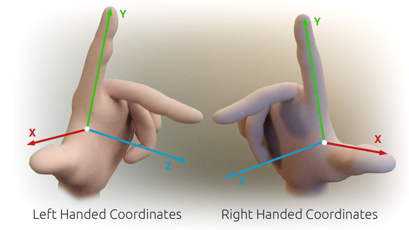
Axes, coordinates and notation

The two perpendicular lines used on a plane are called axes (singular: axis). Conventionally the horizontal axis is labeled x and the vertical axis y; their intersection is the origin, written (0, 0). The first number in an ordered pair measures displacement along the x-axis (the abscissa), while the second measures displacement along the y-axis (the ordinate). Orientation and units are chosen according to context: the axes may be scaled equally to preserve geometric shape, or scaled differently for practical reasons. The same idea extends to three dimensions by adding a z-axis and to higher dimensional spaces by adding coordinates as needed. See coordinate system and location for related concepts.

Algebraic representation and common equations

One of the system's key strengths is the ability to represent geometric objects by algebraic equations. A straight line in the plane can be written as y = mx + b, where m is the slope and b the intercept; a circle centered at the origin with radius r satisfies x^2 + y^2 = r^2. Parabolas, ellipses and hyperbolas all have simple algebraic descriptions in Cartesian coordinates, which makes it straightforward to analyze intersections, tangents and other properties by algebraic manipulation. Typical examples include:

• Line: y = mx + b
• Circle: x^2 + y^2 = r^2
• Parabola: y = ax^2 + bx + c
• Ellipse and hyperbola: quadratic forms in x and y

Plotting solutions of an equation produces a graph: each solution pair corresponds to a point whose coordinates satisfy the equation. This bridging of algebra and geometry led to the development of analytic geometry and later calculus.

Higher dimensions and vectors

The Cartesian approach generalizes naturally to three dimensions by adding a third perpendicular axis, z, so a point is (x, y, z). In higher dimensions, points are tuples (x_1, x_2, ..., x_n) and are commonly treated as vectors. This ties the coordinate system closely to linear algebra: coordinates change under rotations, scalings and shears via matrices. Such vector-based descriptions are essential in physics, computer graphics and engineering simulations. For introductions, see 3D, 4D and dimension topics.

History and development

The system is named after René Descartes, who in the 17th century proposed linking algebra and geometry. His publications showed how to measure positions on a surface using two perpendicular lines and how algebraic equations correspond to geometric curves. This insight, developed in works such as the Discourse on Method and La Géométrie, provided a foundation for analytic geometry and influenced the later formation of calculus and modern mathematics. Further historical context is discussed under Descartes, algebra and Euclidean geometry.

Applications and examples

Cartesian coordinates are used across sciences and engineering. In physics they describe position, velocity and forces; in computer graphics they locate pixels and model 3D scenes; in navigation and cartography they form the basis for map projections and coordinate referencing. In statistics and data analysis, scatter plots use Cartesian axes to reveal relationships between two variables. Simple classroom examples include plotting points, sketching lines and circles, and solving systems of linear equations by graphing. For applied uses see calculus, cartography and computer graphics.

Important distinctions and notable facts

Cartesian coordinates differ from alternative systems such as polar coordinates, where a point is described by radius and angle rather than by orthogonal distances. Choosing the appropriate coordinate system often simplifies problem solving: symmetry around a point suggests polar coordinates, while rectangular symmetry suggests Cartesian. Orthogonality of axes guarantees that distances and angles can be recovered easily when the axes form an orthonormal basis; otherwise coordinate formulas incorporate scale factors. Coordinate transformations and change of basis are central ideas in linear algebra and analytic geometry.

Practical tips and conventions

Common conventions include labeling the rightwards direction on the x-axis positive and the upwards direction on the y-axis positive, though different fields sometimes reverse handedness for convenience. Gridlines, tick marks and consistent units help preserve proportions when plotting. When working algebraically, implicit equations like F(x,y)=0 and parametric forms x(t), y(t) are equivalent ways to represent curves. See further reading on plotting and parametric equations.