Electron cloud (atomic orbital model)
A modern atomic model describing electrons as probability distributions (orbitals) around the nucleus; explains chemical behavior, spectroscopy, and periodic trends.
Overview
The term "electron cloud" is a popular way to describe the probabilistic regions around an atomic nucleus where electrons are most likely to be found. Unlike a classical particle path, the cloud represents a distribution derived from a quantum mechanical wavefunction. The formal concept behind this picture is the atomic orbital, a mathematical function that gives the probability density for an electron's position.
Image gallery
10 Images


Key characteristics and language
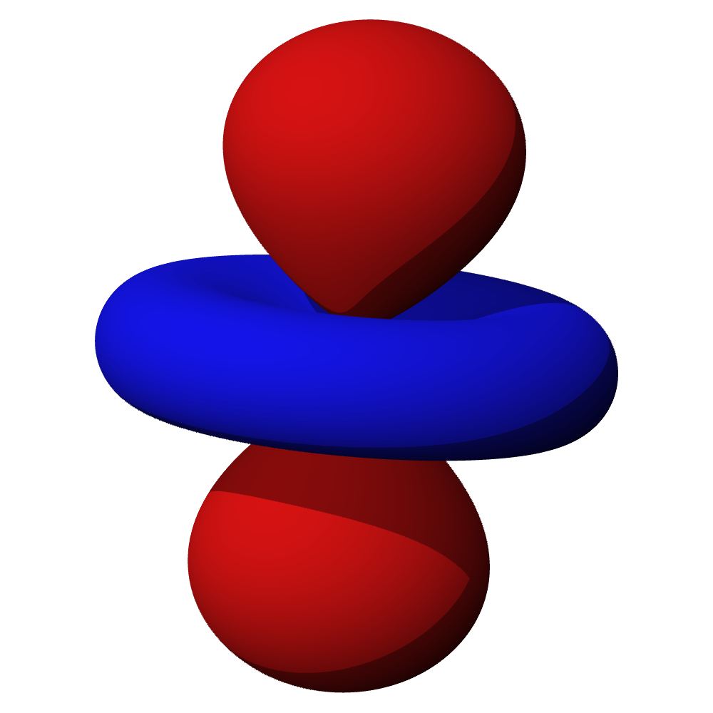
Electron clouds are not literal clouds of smeared charge; they are visualizations of probability density. The wavefunction's squared magnitude yields regions of high and low probability, often drawn as contours or shaded volumes. Atomic structure is described in terms of shells and subshells: principal energy levels (commonly labeled n = 1, 2, 3, … and historically with letters K, L, M, …) and subshells designated s, p, d, f, etc. Each subshell has a characteristic shape and capacity (s: 2, p: 6, d: 10, f: 14) and contributes to an atom's electronic configuration and chemical properties.
Historical development
The electron cloud picture grew out of early 20th‑century work to replace the notion of electrons circling the nucleus in fixed orbits. Niels Bohr's model provided important energy quantization ideas (Bohr), but could not accommodate multi-electron atoms or the wave nature of matter. The modern, wave‑mechanical interpretation was developed in the mid‑1920s by pioneers such as Erwin Schrödinger and Werner Heisenberg; Schrödinger's equation produces orbitals and a probability interpretation popularized by Max Born. Texts and visual models built on this foundation are sometimes called the electron cloud model and arise from the broader framework of quantum mechanics.
How the model is used
Chemists and physicists use orbitals to explain bonding, reactivity, and spectra. The layout of electrons among orbitals underlies the periodic table's structure and recurring chemical behavior (periodic trends). Computational chemistry and spectroscopy both rely on orbital concepts to predict energies and transition probabilities. For hydrogen, the radial distribution of the 1s orbital peaks at about the Bohr radius (approximately 0.529 Å), a distance often cited when comparing simple classical and quantum descriptions (Bohr radius).
Practical examples and notation
- Notation such as 1s, 2p, 3d indicates principal level and subshell; electrons fill these according to the Pauli principle and Hund's rule.
- Orbital shapes: s is roughly spherical, p has two lobes, d and f are more complex; these shapes affect molecular geometry and overlap in bonding.
- Measurements like photoelectron spectroscopy probe orbital energies; calculations solving Schrödinger's equation yield the numerical orbitals used in modeling (Schrödinger, Heisenberg).
Common misconceptions and distinctions
Two frequent misunderstandings are that the electron cloud is a physical smear and that electrons have precise orbits like planets. In reality, the cloud encodes probabilities constrained by principles such as the uncertainty principle; a measurement yields a definite result, but repeated identical preparations produce the distribution described by the orbital. The older Bohr picture retains pedagogical value for introducing quantized energies, but the cloud (orbital) model gives a more accurate and generally applicable description of atomic structure and chemical behavior.
For further reading on formal definitions and mathematical formulations see introductory treatments of atomic orbitals, basic texts on quantum mechanics, and materials connecting orbitals to the periodic table and spectroscopy. Historical surveys often discuss the transition from Bohr's ideas (Bohr) to wave mechanics (Schrödinger, Heisenberg) and modern interpretations of measurement and probability.
Additional resources: introductory visualizations and computational examples are available through educational collections and simulation tools that implement orbital plotting and electron density mapping (electron cloud model, Bohr radius).
Related articles
Author
AlegsaOnline.com Electron cloud (atomic orbital model) Leandro Alegsa
URL: https://en.alegsaonline.com/art/30730