
RLC Circuit — Theory, Components, Damping, and Applications
Comprehensive overview of RLC circuits: series and parallel forms, governing equations, damping and resonance, energy flow, practical applications and distinctions for engineers and students.
Overview
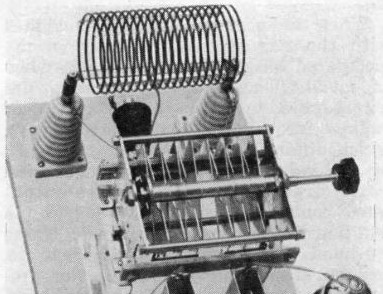
An RLC circuit is an electrical network that contains a resistor (R), an inductor (L), and a capacitor (C) connected in series or in parallel. Such circuits are fundamental models for oscillatory electrical behavior: they store energy alternately in the capacitor’s electric field and the inductor’s magnetic field while a resistor dissipates energy as heat. The basic dynamics of charge and current in an RLC circuit are governed by a second-order linear differential equation that determines whether the response is oscillatory or overdamped.
Image gallery
2 Images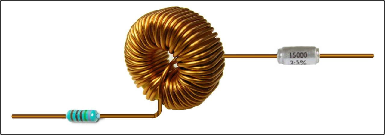
Main parts and energy
Each component plays a distinct role. The resistor converts electrical energy into thermal energy and sets the rate at which oscillations decay. The inductor stores magnetic energy proportional to the square of the current. The capacitor stores electric energy proportional to the square of the charge. In a lossless LC circuit the total electromagnetic energy is constant; with R present the total energy U = 1/2 L i^2 + 1/2 q^2/C decreases over time because dU/dt = −i^2 R. That loss is the physical cause of damping.
Governing equations and regimes
For a series RLC circuit the standard form is L d^2q/dt^2 + R dq/dt + q/C = 0, where q(t) is charge and i = dq/dt is current. The undamped natural angular frequency is ω0 = 1/√(LC). The damping coefficient is α = R/(2L). The response falls into three regimes depending on R: underdamped (α < ω0) where the circuit oscillates with exponentially decaying amplitude, critically damped (α = ω0) where the system returns to equilibrium in the shortest non-oscillatory way, and overdamped (α > ω0) where the return is slow and non-oscillatory. The critical resistance for a series circuit is Rcrit = 2√(L/C). The quality factor Q = ω0 L / R quantifies selectivity and energy loss per cycle.
Resonance and frequency response
At resonance (ω = ω0) a series RLC circuit presents its minimum impedance and can support large currents limited primarily by R; a parallel RLC shows maximum impedance at resonance. Resonant behavior underlies radio tuning, narrowband filters, and many measurement techniques. The bandwidth Δω of the resonant peak relates to Q by Q = ω0 / Δω. Engineers use this relation when designing filters or oscillators to control selectivity and transient settling time.
Applications and examples
- Tuning circuits in radios and RF receivers — selecting desired frequencies while rejecting others. Energy storage and transfer between L and C enable sustained oscillations when energy is periodically supplied.
- Filters and equalizers — low-pass, band-pass, and notch filters are built from RLC sections to shape frequency response.
- Transient analysis in power systems and signal-processing — RLC models describe how circuits respond to pulses and step inputs, including damping of unwanted oscillations. Oscillations appear in both intentional and parasitic forms.
- Pulse shaping and timing in analog circuits, and impedance matching in RF design to optimize energy transfer.
Historical notes and practical distinctions
RLC models derive from the 19th-century development of electrical theory: capacitors (Leyden jar) and inductors (coils) were studied as scientists formalized Maxwell’s laws and circuit analysis. In practice, ideal components are approximations: real inductors have winding resistance and parasitic capacitance; capacitors have leakage and equivalent series resistance (ESR). Design tradeoffs involve balancing R to obtain desired damping: too low R gives high Q and slow settling, too high R broadens response and wastes energy. Simulation and measurement tools help determine appropriate component values for a target transient or frequency response.
Key distinctions and notable facts
Distinguish series from parallel configurations: series RLC emphasizes current-driven resonance and a single resonant impedance minimum, while parallel networks emphasize voltage-driven resonance and a maximum in impedance. In power electronics and high-frequency circuits, parasitic elements can create unintended RLC resonances that must be mitigated. Understanding the interplay of L, C, and R is central to designing stable amplifiers, filters, oscillators, and control systems. Amplitude decay, phase shift, and energy dissipation are measurable consequences of these component interactions.
Related articles
Author
AlegsaOnline.com RLC Circuit — Theory, Components, Damping, and Applications Leandro Alegsa
URL: https://en.alegsaonline.com/art/83192