
Surface integral
An explanation of surface integrals: definitions, parametrization and computation, scalar vs vector integrals (flux), historical context, common applications in physics and engineering, and practical distinctions.
Surface integrals extend the idea of integrating a function over an interval or a planar region to integrating over a two-dimensional surface embedded in three-dimensional space. They come in two closely related forms: integrals of scalar fields (which accumulate a quantity distributed across the surface, such as mass or area-weighted density) and integrals of vector fields (most often interpreted as flux through the surface). A surface integral can be thought of as a double integral over a curved sheet, and it requires a description of the surface and a rule for measuring the area of infinitesimal patches.
Image gallery
1 Image
Basic description and parametrization
To compute a surface integral one generally parametrizes the surface by a smooth map r(u,v) from a domain D in the plane to three-dimensional space. For a scalar function f defined on the surface, the surface integral is written in parametric form as a double integral over D of f(r(u,v)) times the local area element, which is the magnitude of the cross product of the partial derivatives: |r_u × r_v|. For a vector field F the surface integral measuring flux is ∬_S F · n dS, where n is a unit normal and dS is the area element. In parametric coordinates this becomes ∬_D F(r(u,v)) · (r_u × r_v) dudv, with the sign depending on the chosen orientation.
Characteristics and computational steps
- Choose a parametrization r(u,v) of the surface and determine the parameter domain D.
- For scalar integrals: evaluate f(r(u,v)) and multiply by |r_u × r_v|, then integrate over D.
- For flux integrals: evaluate the vector field at points on the surface and take the dot product with r_u × r_v (or with the unit normal), then integrate over D.
- Pay attention to orientation: reversing the normal flips the sign of a vector (flux) integral but does not affect a scalar surface integral of area or mass.
Applications and examples
Surface integrals appear throughout mathematics, physics and engineering. Typical uses include computing the surface area of a curved object, the total mass of a thin shell with surface density, and the flux of a vector field (such as an electric or fluid flow) through a surface. In electromagnetism the flux of the electric field through a closed surface relates to enclosed charge (Gauss's law). In fluid mechanics the flux across a surface describes the rate at which fluid crosses a boundary. In differential geometry surface integrals are central to defining integrals of differential forms on manifolds.
Historical context and related theorems
Surface integrals developed as part of the 19th-century extension of calculus to higher dimensions and curved domains. They are closely connected with fundamental integral theorems: Green's theorem in the plane, Stokes' theorem (relating a surface integral of the curl of a vector field to a line integral around the boundary), and the divergence theorem (relating flux through a closed surface to a volume integral of divergence). These theorems organize many computations and provide deep relationships between local differential properties and global integral quantities.
Practical distinctions and notable facts
Not all surfaces are orientable: on a nonorientable surface (for example, a Möbius strip) a global choice of continuous normal vector field is impossible, so vector-field flux integrals require care and are typically defined only locally or with additional structure. Closed surfaces (those without boundary) are often used when discussing total flux, while open surfaces require specification of an orientation and may have boundary integrals associated via Stokes' theorem. Numerically, surface integrals are approximated by discretizing the surface into small panels and summing contributions; in analytic problems, symmetry and clever parametrizations simplify the calculation.
Further reading
- Introductory notes on surface integration
- Parametrization techniques for surfaces
- Scalar and vector surface integrals explained
- Computing area and mass of surfaces
- Flux and Gauss's law applications
- Stokes' theorem and its uses
- Surface integrals in electromagnetism
- Numerical methods for surface integrals
Terms and definitions
In integration over surfaces, parameterizations of the surface take the place of the integration variable and surface elements take the place of the infinitesimal (infinitesimal) interval width  .
.
Parameterization
As a two-dimensional set, a surface can be represented (parameterized) as a function of two variables. If  a set whose boundary contains no double points, is continuously differentiable, is not infinitely long, and further φ
  a mapping from
  into
into  , we say that φ is parametrization of the surface
  , if
, if  . At this point, it is worth noting that much of the difficulty in dealing with surface integrals is related to the parametrization. It is not clear a priori that different parameterizations produce the same value for the integral. A change of coordinates for surface integrals is not trivial and is consequently motivation for the use of differential forms.
general, a surface in with two parameters  and
and  in the following form:
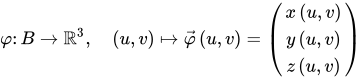
On the surface φ the sets of curves  resp.
resp.  form
form  the coordinate lines. These cover the surface with a coordinate mesh, with two coordinate lines running through each point. Thus, each point on the surface has unique coordinates
  .
.
Example 1: Parameter representation
The surface of a sphere of radius  can be parameterized as follows: is the rectangle
 ![[0,\pi ]\times [0,2\pi ]](https://www.alegsaonline.com/image/0d0ac12bb0cbbae24d6597c057f4f8ee645e571f.svg) and
and
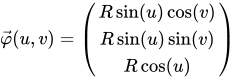 .
.
This parametrization satisfies the spherical equation  (see also spherical coordinates). is here the polar angle (usually
  or θ
or θ  ) and the azimuth angle (usually
  denoted φ {\displaystyle
 or ϕ ).
Example 2: Explicit representation
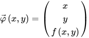
If  a function and the surface is
  given in the form , then
  and are
  the two parameters; thus the parametrization of the surface looks like this:
Surface element
If in the one-dimensional case the represents the width of an infinitesimal interval, it is natural to replace it in the two-dimensional case by the area of an infinitesimal piece of surface  . By the parametrization described in the previous section, one can put two tangents to any point on the surface (see also: curvilinear coordinates): once the tangent that arises if one leaves constant and varies minimally, and once with swapped variables. That is, two tangents to the two coordinate lines at the point under consideration . These tangents can be expressed by two infinitesimal tangent vectors (let φ the parameterized form of the surface):
 and ∂
and ∂
In the following, the compact notation is used for the partial derivatives:
 and φ
and φ 
If these tangents are not parallel at any point on the surface, we speak of a regular parametrization. The cross product of the tangent vectors is then a vector whose length is not equal to zero.

The two tangent vectors lie in the tangent plane of the surface at the point under consideration. The area of the parallelogram spanned by the two tangent vectors is now just equal to the magnitude of their cross product.
Now if φ is  a regular parametrization of the surface, we define:
- Scalar surface element

- Vector surface element
 with the unit normal vector of the area element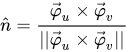
According to the properties of the cross product, the vector surface element is perpendicular to the surface, its magnitude is just equal to the size of the infinitesimal surface piece.
In the form presented above, the vector surface element is not well-defined, since its direction depends on whether one wants φ  or φ
or φ  computed. The two possibilities are antiparallel to each other. When considering closed surfaces, one usually agrees that the outward facing vector surface element should be used.
Example 1: Parameter representation
The surface of the sphere of radius R can be parameterized by the polar angle and the azimuthal angle as shown above. The surface element is obtained from the following calculation:
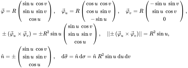
For the normal vector, two solutions are possible (  ), depending on the order of φ
  and φ
and φ  in the cross product. Typically, one chooses here the positive solution where
  points away from the convex surface of the sphere (so-called "outer normal").
Example 2: Explicit representation
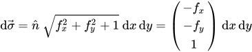
If the area is of the form , then the area element is expressed by the differentials of the coordinates , .


Thus, area element and vector area element are the same:

Projection on surface with known surface element
We assume in the following that a surface  with its surface element
  and associated normal vector
  is known. FOR EXAMPLE.
- xy-plane:
and 
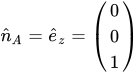
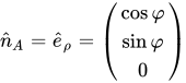
- Sheath area of a circular cylinder with radius ρ
 :
:
and 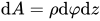
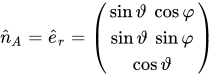
- Spherical surface with radius
 :
:
and 
For another surface with normal vector  , find the surface element be determined. The area is
 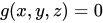 given approximately by and thus the normal vector is equal to
  .
.
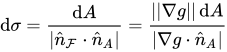
We now project along onto . Then the area elements can be calculated using  for
for  link:
link:
Each straight line along the normal vectors may intersect the surface only once. Otherwise, one must divide the surface into smaller surfaces  , whose projection is then unique, or choose a different footprint
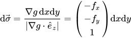
The vectorial area element is:

Example 1
Let a surface the form be given, then  and so:

This surface is now projected into the  plane with and
  ; where

Example 2
We are looking for the area element of a body of revolution about the  -axis with ρ
  , so
, so  .
.

By projecting onto the lateral surface of a circular cylinder with radius ρ the area element is obtained:


The integrals
With the parameterizations and the surface elements, one can now define the surface integrals. These multidimensional integrals are Lebesgue integrals, but in most applications they can be calculated as multiple Riemann integrals.
The scalar surface integral
The scalar surface integral of a scalar function  over a surface with regular parametrization φ
  with is defined as
 .
.
For example, if we set  , then the scalar surface integral is simply the area of the surface.
Example: Surface area of a sphere
With the area element for spherical coordinates

obtained for the surface area a sphere of radius :
 .
.
The vectorial surface integral
The vector surface integral of a vector-valued function  over a surface with regular parametrization φ with is defined as
 .
.
A descriptive notion of this integral occurs via the flow  a vector field
  through the surface : The quantity
  indicates, what contribution to the total flux
  the infinitesimal-small surface vector
  provides; namely, how much of
  flows through the surface piece The flow is maximal when the vector field parallel to the surface normal and zero, if perpendicular to that is, tangent to the surface - then "flows" along the surface, but not through it.
Example: Flow of a vector field through a spherical surface
Given a radially symmetric vector field
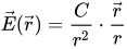
With a constant  , the location vector
  and its magnitude . The vector
  is thus a unit vector in the direction of the location vector. In physics, for example, the electric field of a point charge
  at the coordinate origin is of this form: see Coulomb's law.
For symmetry reasons one uses spherical coordinates. The vector surface element  for a sphere with radius and center at the coordinate origin is
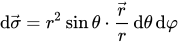 .
.
For the flux of the vector field  through the surface a sphere of radius obtain:
 .
.
The flux the vector field through the sphere surface is thus independent of the sphere radius . For the physical example of the electric field of a point charge, this result is a special case of Gauss' law of electrostatics.
Questions and answers
Q: What is a surface integral in mathematics?
A: A surface integral is a definite integral taken over a surface, which may be a curve set in space.
Q: What is the difference between a line integral and a surface integral?
A: A line integral allows one to integrate over an arbitrary curve of one dimension, while a surface integral can be thought of as a double integral integrating over a two-dimensional surface.
Q: What can be integrated over a surface?
A: Given a surface, one may integrate over its scalar fields or its vector fields.
Q: What are scalar fields?
A: Scalar fields are functions which return numbers as values.
Q: What are vector fields?
A: Vector fields are functions which return vectors as values.
Q: What are the applications of surface integrals in physics?
A: Surface integrals have applications in physics, particularly with the classical theory of electromagnetism.
Q: How can surface integrals be used in electromagnetism?
A: Surface integrals are useful in calculating magnetic flux or electric flux through a closed surface.
Related articles
Author
AlegsaOnline.com Surface integral Leandro Alegsa
URL: https://en.alegsaonline.com/art/95155