Student's t-distribution

The Student t-distribution (also Student t-distribution or t-distribution for short) is a probability distribution developed in 1908 by William Sealy Gosset and named after his pseudonym Student.

Gosset had found that the standardized estimator of the sample mean of normally distributed data is no longer normally distributed but -distributed when the variance of the characteristic needed to standardize the mean is unknown and must be estimated with the sample variance. Its -distribution allows - especially for small sample sizes - to calculate the distribution of the difference from the sample mean to the true population mean.

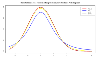
The values depend on the significance level as well as on the sample size and determine the confidence interval and thus the significance of the estimate of the mean. The distribution becomes narrower with increasing and transitions to the normal distribution for $n\to \infty$ (see graph on the right). Hypothesis tests that use the distribution are called t-tests.

The derivation was first published in 1908, when Gosset was working at the Guinness brewery in Dublin. Since his employer did not permit its publication, Gosset published it under the pseudonym Student. The t-factor and the associated theory were first proven by the work of R. A. Fisher, who called the distribution Student's distribution.

However, the distribution also appears in earlier publications by other authors. It was first derived in 1876 by Jacob Lüroth as an a posteriori distribution in the treatment of a problem of the equalization calculus, and in 1883 in a similar context by Edgeworth.

Densities of -distributed random variables

Definition

A continuous random variable satisfies the student distribution with if it has probability density

$f_{n}(x)={\frac {\Gamma \left({\frac {n+1}{2}}\right)}{{\sqrt {n\pi }}~\Gamma \left({\frac {n}{2}}\right)}}\left(1+{\frac {x^{2}}{n}}\right)^{-{\frac {n+1}{2}}}\quad \mathrm {f{\ddot {u}}r} \quad -\infty <x<+\infty$

owns. Thereby is

$\Gamma(x)=\int\limits_{0}^{+\infty}t^{x-1}e^{-t}\operatorname{d}t$

the gamma function. For natural numbers applies in particular (here the factorial of )

$\Gamma (n+1)=n!,\quad \Gamma \left(n+{\tfrac {1}{2}}\right)={\frac {(2n)!}{n!\,4^{n}}}\,{\sqrt {\pi }}.$

Alternatively, the distribution with degrees of freedom can also be defined as the distribution of size

$t_{n}\equiv {\frac {Z}{\sqrt {\chi _{n}^{2}/n}}}$ ,

where is a standard normally distributed random variable and χ $\chi_n^2$ is a chi-squared distributed random variable with degrees of freedom, independent of

Distribution

The distribution function can be expressed in closed form as

$F_{n}(t)=I\left({\frac {t+{\sqrt {t^{2}+n}}}{2{\sqrt {t^{2}+n}}}},{\frac {n}{2}},{\frac {n}{2}}\right)$

or as

$F_{n}(t)={\frac {1}{2}}\left(1+{\frac {t}{|t|}}I\left({\frac {t^{2}}{t^{2}+n}},{\frac {1}{2}},{\frac {n}{2}}\right)\right)$

with

$I(z,a,b)={\frac {1}{B(a,b)}}\int _{0}^{z}t^{a-1}(1-t)^{b-1}\mathrm {d} t,$

where represents the beta function.

F_n(t) calculates the probability that a random variable f_n(x) distributed according to receives a value less than or equal to

Properties

Let be a -distributed random variable with degrees of freedom and density f_n(x) .

Turning Points

The density has inflection points at

$x=\pm\,\sqrt{\frac{n}{n+2}}.$

Median

The median is

$\tilde{x}=0.$

Mode

The mode results in

$x_{D}=0.$

Symmetry

The Student's distribution is symmetric about 0.

Expected value

For the expected value we get for n>1

$\operatorname{E}(X)=0.$

The expected value for does not exist. n=1

Variance

The variance for results in

$\operatorname{Var}(X)=\frac{n}{n-2}.$

Skew

The skewness is for n>3

$\operatorname{v}(X)=0.$

Cambers

For kurtosis kurtosis β $\beta _{2}$ and excess kurtosis γ $\gamma_2$ we obtain for n>4

$\operatorname{\beta_2}(X)=\frac{\mu_4}{\mu_2^2}=\frac{3n-6}{n-4},\qquad \operatorname{\gamma_2}(X)=\frac{\mu_4}{\mu_2^2}-3=\frac{6}{n-4}.$

Moments

For the -th moments $m_k=\operatorname{E}(X^k)$ and the -th central moments μ $\mu_k=\operatorname{E}([X-\operatorname{E}(X)]^k)$ holds:

$m_{k}=\mu _{k}=0,{\text{ falls }}n>k{\text{ und }}k{\text{ ungerade}}$

$m_{k}=\mu _{k}=n^{{k/2}}\cdot {\frac {1\cdot 3\cdot 5\cdot 7\dotsm (k-1)}{(n-2)\cdot (n-4)\cdot (n-6)\dotsm (n-k)}},{\text{ falls }}n>k{\text{ und }}k{\text{ gerade}}$

Relationship to beta distribution

The integral

$\int _{0}^{z}t^{a-1}(1-t)^{b-1}\mathrm {d} t$

is the incomplete beta function

$B(z;a,b),$

where

$B(a,b)=B(1;a,b)$ establishes the connection to the complete beta function. Then for t>0

$F_{n}(t)={\tfrac {1}{2}}+{\tfrac {1}{2}}I(z,{\tfrac {1}{2}},{\tfrac {n}{2}})={\tfrac {1}{2}}+{\tfrac {1}{2}}{\frac {B(z_{t};{\tfrac {1}{2}},{\tfrac {n}{2}})}{B(1;{\tfrac {1}{2}},{\tfrac {n}{2}})}}$

with

$z_{t}={\frac {t^{2}}{t^{2}+n}}.$

If t goes to infinity, $z_{t}$ to 1. In the limiting case, the numerator and denominator of the above fraction are the same, i.e., we get:

$F_{n}(t)={\tfrac {1}{2}}+{\tfrac {1}{2}}I(z_{t},{\tfrac {1}{2}},{\tfrac {n}{2}})\rightarrow {\tfrac {1}{2}}+{\tfrac {1}{2}}=1$

Non-central t-distribution

The size

${\frac {Z+\delta }{\sqrt {\chi _{n}^{2}/n}}}$

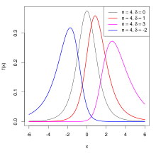
with $Z\sim {\mathcal {N}}(0,1)$ and δ $\delta$ as non-centrality parameter follows the so-called non-central -distribution. This distribution is mainly used to determine the β-error in hypothesis tests with -distributed test variable. Its probability density is:

$f(x)={\frac {n^{n/2}n!e^{-\delta ^{2}/2}}{2^{n}\Gamma \left(n/2\right)(x^{2}+n)^{(n+1)/2}}}\left({\frac {{\sqrt {2}}\delta x}{\sqrt {x^{2}+n}}}{\frac {_{1}{\mathcal {F}}_{1}\left(n/2+1,3/2,{\frac {(\delta x)^{2}}{2(x^{2}+n)}}\right)}{\Gamma \left((n+1)/2\right)}}+{\frac {_{1}{\mathcal {F}}_{1}\left((n+1)/2,1/2,{\frac {(\delta x)^{2}}{2(x^{2}+n)}}\right)}{\Gamma \left(n/2+1\right)}}\right)$

The parenthesis with the sum of hypergeometric functions can be written a bit simpler still, resulting in a shorter alternative expression for the density:

$f(x)={\frac {2^{n}n^{n/2+1}\Gamma \left((n+1)/2\right)}{\pi (x^{2}+n)^{(n+1)/2}}}e^{-\delta ^{2}/2}H_{-n-1}\left(-{\frac {\delta x}{{\sqrt {2}}{\sqrt {x^{2}+n}}}}\right),$

where $H_{-n-1}\left(z\right)$ represents a Hermitian polynomial with negative index with $H_{-n-1}\left(0\right)={\frac {\sqrt {\pi }}{2^{n+1}\Gamma \left(n/2+1\right)}}$ .

The expected value for

${\frac {\delta {\sqrt {n}}\Gamma \left((n-1)/2\right)}{{\sqrt {2}}\Gamma \left(n/2\right)}}$

and the variance (for

${\frac {(1+\delta ^{2})n}{n-2}}-{\frac {\delta ^{2}n\Gamma \left((n-1)/2\right)^{2}}{2\Gamma \left(n/2\right)^{2}}}.$

With δ $\delta =0$ we obtain the characteristics of the central distribution.

Some densities of non-central distributions

Relationship with other distributions

Relationship to Cauchy distribution

For n=1 and with Γ $\Gamma(1/2)=\sqrt{\pi}$ the Cauchy distribution results as a special case from the Student's distribution.

Relationship to Chi-Square Distribution and Standard Normal Distribution

The distribution describes the distribution of an expression

$t_{n}\equiv {\frac {{\mathcal {N}}(0,1)}{\sqrt {\frac {\chi _{n}^{2}}{n}}}},$

where denotes ${\mathcal {N}}(0,1)$ a standard normally distributed and χ $\chi_n^2$ denotes a chi-squared distributed random variable with degrees of freedom. The numerator variable must be independent of the denominator variable. The density function of the distribution is then symmetric with respect to its expected value $0$ . The values of the distribution function are usually available in tabular form.

Distribution with heavy edges

The distribution belongs to the distributions with heavy edges.

Approximation by the normal distribution

As the number of degrees of freedom increases, the distribution values of the distribution can be approximated using the normal distribution. As a rule of thumb, from 30 degrees of freedom, the distribution function can be approximated by the normal distribution.

Use in mathematical statistics

Various estimators are -distributed.

If the independent random variables $X_1, X_2, \dotsc, X_n$ are identically normally distributed with expected value μ $\mu$ and standard deviation σ $\sigma$ , it can be proved that the sample mean is

${\overline {X}}={\frac {1}{n}}\sum _{i=1}^{n}X_{i}$

and the sample variance

$S^{2}={\frac {1}{n-1}}\sum _{i=1}^{n}(X_{i}-{\overline {X}})^{2}$

are stochastically independent.

Because the random variable ${\tfrac {{\overline {X}}-\mu }{\sigma /{\sqrt {n}}}}$ has a standard normal distribution and $(n-1)\, S^2/\sigma^2$ follows a chi-squared distribution with n-1 degrees of freedom, it follows that the quantity

$t_{n-1}={\frac {{\overline {X}}-\mu }{S/{\sqrt {n}}}}={\frac {{\overline {X}}-\mu }{S/{\sqrt {n}}}}\cdot {\frac {\sigma }{\sigma }}={\frac {{\overline {X}}-\mu }{\sigma /{\sqrt {n}}}}\cdot {\frac {\sigma }{S}}={\frac {{\overline {X}}-\mu }{\sigma /{\sqrt {n}}}}/\left({\frac {S}{\sigma }}\right)={\frac {{\overline {X}}-\mu }{\sigma /{\sqrt {n}}}}/{\sqrt {\chi _{n-1}^{2}/(n-1)}}$

by definition is -distributed with n-1 degrees of freedom.

So the distance of the measured mean from the mean of the population is distributed as $t_{n-1} S/\sqrt{n}$ . This is then used to calculate the 95 % confidence interval for the mean μ $\mu$ to be

${\overline {x}}-t\cdot S/{\sqrt {n}}\leq \mu \leq {\overline {x}}+t\cdot S/{\sqrt {n}},$

where is determined by $F_{n-1}(t)=0{,}975$ This interval is somewhat larger for $n < \infty$ slightly larger than the one that would have resulted with known σ $\sigma$ from the distribution function of the normal distribution at the same confidence level $\left(\mu \in \left[{\overline {x}}\pm 1{,}96\cdot {\tfrac {\sigma }{\sqrt {n}}}\right]\right)$ .

Density derivation

The probability density of the distribution can be derived from the joint density of the two independent random variables and χ $\chi^2_n$ which are standard normal and chi-squared distributed, respectively:

$f_{Z,\chi _{n}^{2}}(z,y)={\frac {e^{-{\frac {1}{2}}z^{2}}}{\sqrt {2\pi }}}\cdot {\frac {y^{{\frac {n}{2}}-1}e^{-{\frac {1}{2}}y}}{2^{\frac {n}{2}}\Gamma ({\frac {n}{2}})}}$

With the transformation

$t=z/{\sqrt {y/n}},v=y$

get the joint density of $T=Z/\sqrt{\chi^2_n/n}$ and χ $\chi^2_n$ , where $-\infty <t<\infty$ <

The Jacobian determinant of this transformation is:

$\det\frac{\partial(z,y)}{\partial(t,v)}=\begin{vmatrix} \sqrt{\frac{v}{n}}&0\\ \Diamond&1 \end{vmatrix}=\sqrt{\frac{v}{n}}$

The value $\Diamond$ is unimportant because it is multiplied by 0 when calculating the determinant. The new density function is thus written

$f_{T,\chi^2_n}(t,v)=\frac{e^{-\frac 12 v \frac{t^2}n}}{\sqrt{2\pi}} \cdot \frac{1}{2^\frac n2 \Gamma(\frac n2)}v^{\frac n2-1}e^{-\frac 12v}\cdot\sqrt{\frac{v}{n}}.$

We are now looking for the marginal distribution as an f_n(t) integral over the variable of no interest :

$f_{n}(t)=\int \limits _{0}^{\infty }f_{T,\chi _{n}^{2}}(t,v)\,dv={\frac {1}{{\sqrt {n\pi }}\,2^{(n+1)/2}\Gamma (n/2)}}\int \limits _{0}^{\infty }v^{(n-1)/2}e^{-v(1+t^{2}/n)/2}\,dv={\frac {\Gamma \left({\frac {n+1}{2}}\right)}{{\sqrt {n\pi }}\Gamma \left({\frac {n}{2}}\right)}}\left(1+{\frac {t^{2}}{n}}\right)^{-{\frac {n+1}{2}}}$

Selected quantiles of the t-distribution

Tabulated are values for various degrees of freedom and common probabilities (0.75 to 0.999), whereof holds:

$P_{{{\text{einseitig}}}}=F_{n}(t)=P(T_{n}\leq t)$

Due to the mirror symmetry of the density, one only needs to adjust the probability scale for the case of the interval bounded symmetrically on both sides. Thereby the probabilities decrease for the same because the integration interval is - t reduced by cutting away the range from $-\infty$ to

$P_{{{\text{zweiseitig}}}}=F_{n}(t)-F_{n}(-t)=P(-t<T_{n}\leq t)=2P_{{{\text{einseitig}}}}-1$

If in a sample observations are made and parameters are estimated from the sample , then n=N-m the number of degrees of freedom.

To the number of degrees of freedom in the first column and the significance level α $\alpha$ (represented as $1-\alpha$ second row), in each cell of the following table the value of the (one-sided) quantile $t_{n,\alpha}$ , corresponding to DIN 1319-3, is given. This satisfies the following equations for the density of $f_{n}$ the t_n distribution:

One-sided: $\int_{-\infty}^{t_{n,\alpha}}f_n(x)\,\mathrm{d}x=1-\alpha$

Two-sided: $\int_{-t_{n,\alpha/2}}^{t_{n,\alpha/2}}f_n(x)\,\mathrm{d}x=1-\alpha$

So, for example, with n=4 and α $\alpha = 0{,}05$ find the values of 2.776 (two-sided) or 2.132 (one-sided).

The quantile function of the distribution x_p is the solution of the equation $p=F(x_p|m,\,n)$ and thus in principle can be calculated via the inverse function. Concretely applies here

$x_{p}={\frac {{\sqrt {n}}\left(2I^{-1}(p,{\frac {n}{2}},{\frac {n}{2}})-1\right)}{2{\sqrt {\left(1-I^{-1}(p,{\frac {n}{2}},{\frac {n}{2}})\right)\cdot I^{-1}(p,{\frac {n}{2}},{\frac {n}{2}})}}}}$

with $I^{{-1}}$ as inverse of the regularized incomplete beta function. This value x_p is entered in the quantile table under the coordinates p and n.

For few values (1,2,4) the quantile function simplifies:

$n=1:x_{p}=\operatorname {tan} (\pi (p-1/2))$

$n=2:x_{p}=(p-1/2){\sqrt {\frac {2}{p(1-p)}}}$

$n=4:x_{p}={\sqrt {{\frac {2\cos \left({\frac {1}{3}}\arccos \left(2{\sqrt {p(1-p)}}\,\right)\right)}{\sqrt {p(1-p)}}}-4}}$

Table of some t-quantiles

→ Main article: Quantile table

NumberDegrees of freedom n	P for two-sided confidence interval
	0,5	0,75	0,8	0,9	0,95	0,98	0,99	0,998
	P for one-sided confidence interval
	0,75	0,875	0,90	0,95	0,975	0,99	0,995	0,999
1	1,000	2,414	3,078	6,314	12,706	31,821	63,657	318,309
2	0,816	1,604	1,886	2,920	4,303	6,965	9,925	22,327
3	0,765	1,423	1,638	2,353	3,182	4,541	5,841	10,215
4	0,741	1,344	1,533	2,132	2,776	3,747	4,604	7,173
5	0,727	1,301	1,476	2,015	2,571	3,365	4,032	5,893
6	0,718	1,273	1,440	1,943	2,447	3,143	3,707	5,208
7	0,711	1,254	1,415	1,895	2,365	2,998	3,499	4,785
8	0,706	1,240	1,397	1,860	2,306	2,896	3,355	4,501
9	0,703	1,230	1,383	1,833	2,262	2,821	3,250	4,297
10	0,700	1,221	1,372	1,812	2,228	2,764	3,169	4,144
11	0,697	1,214	1,363	1,796	2,201	2,718	3,106	4,025
12	0,695	1,209	1,356	1,782	2,179	2,681	3,055	3,930
13	0,694	1,204	1,350	1,771	2,160	2,650	3,012	3,852
14	0,692	1,200	1,345	1,761	2,145	2,624	2,977	3,787
15	0,691	1,197	1,341	1,753	2,131	2,602	2,947	3,733
16	0,690	1,194	1,337	1,746	2,120	2,583	2,921	3,686
17	0,689	1,191	1,333	1,740	2,110	2,567	2,898	3,646
18	0,688	1,189	1,330	1,734	2,101	2,552	2,878	3,610
19	0,688	1,187	1,328	1,729	2,093	2,539	2,861	3,579
20	0,687	1,185	1,325	1,725	2,086	2,528	2,845	3,552
21	0,686	1,183	1,323	1,721	2,080	2,518	2,831	3,527
22	0,686	1,182	1,321	1,717	2,074	2,508	2,819	3,505
23	0,685	1,180	1,319	1,714	2,069	2,500	2,807	3,485
24	0,685	1,179	1,318	1,711	2,064	2,492	2,797	3,467
25	0,684	1,178	1,316	1,708	2,060	2,485	2,787	3,450
26	0,684	1,177	1,315	1,706	2,056	2,479	2,779	3,435
27	0,684	1,176	1,314	1,703	2,052	2,473	2,771	3,421
28	0,683	1,175	1,313	1,701	2,048	2,467	2,763	3,408
29	0,683	1,174	1,311	1,699	2,045	2,462	2,756	3,396
30	0,683	1,173	1,310	1,697	2,042	2,457	2,750	3,385

40	0,681	1,167	1,303	1,684	2,021	2,423	2,704	3,307
50	0,679	1,164	1,299	1,676	2,009	2,403	2,678	3,261
60	0,679	1,162	1,296	1,671	2,000	2,390	2,660	3,232
70	0,678	1,160	1,294	1,667	1,994	2,381	2,648	3,211
80	0,678	1,159	1,292	1,664	1,990	2,374	2,639	3,195
90	0,677	1,158	1,291	1,662	1,987	2,368	2,632	3,183
100	0,677	1,157	1,290	1,660	1,984	2,364	2,626	3,174

200	0,676	1,154	1,286	1,653	1,972	2,345	2,601	3,131
300	0,675	1,153	1,284	1,650	1,968	2,339	2,592	3,118
400	0,675	1,152	1,284	1,649	1,966	2,336	2,588	3,111
500	0,675	1,152	1,283	1,648	1,965	2,334	2,586	3,107

$\infty$	0,674	1,150	1,282	1,645	1,960	2,326	2,576	3,090

Questions and Answers

Q: What is Student's t-distribution?

A: Student's t-distribution is a probability distribution which was developed by William Sealy Gosset in 1908. It describes samples drawn from a full population, and the larger the sample size, the more it resembles a normal distribution.

Q: Who developed Student's t-distribution?

A: William Sealy Gosset developed Student's t-distribution in 1908. He used the pseudonym "Student" when he published the paper describing it.

Q: What are some of the uses of Student's t-distribution?

A: The Student's t-distribution plays a role in many widely used statistical analyses, including the Student's t-test for assessing the statistical significance of differences between two sample means, constructing confidence intervals for differences between two population means, and linear regression analysis. It also arises in Bayesian analysis of data from a normal family.

Q: How does sample size affect the shape of a t-distribution?

A: The larger the sample size, the more closely it will resemble a normal distribution. For each different sample size there is an associated unique t-distribution that describes it.

Q: Is there any relation between Student’s T Distribution and Normal Distribution?

A: Yes - while normal distributions describe full populations, student’s T Distributions describe samples drawn from those populations; as such they share similarities but differ depending on their respective sizes. As mentioned above, larger samples tend to look more like normal distributions than smaller ones do.

Q: Is there any other name for this type of distribution?

A: No - this type of distribution is known as "Student's T Distribution," named after its developer William Sealy Gosset who used his pseudonym "Student" when publishing his paper about it.