Square root

The square root of a number is a value that, when squared, yields the original number. This article explains definitions, notation, real and complex roots, computation methods, and common applications.

Author: Leandro Alegsa Created: November 13, 2022 Updated: May 6, 2026

Overview and definition

The square root of a number x is any number y such that y·y = x. For nonnegative real x there is a unique nonnegative square root, commonly written with the radical sign as √x. That nonnegative value is called the principal square root. For example, 3 is a square root of 9 because 3×3 = 9; the principal square root of 9 is written √9 = 3. The single value 0 is the only square root of 0. An illustration: ${\sqrt {x}}$

Image gallery

5 Images

en.wikipedia.org · Public domain

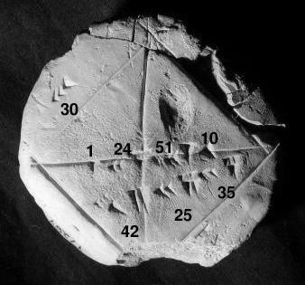
Basic properties and distinctions

Square roots interact with arithmetic in several useful ways, but with important caveats. For nonnegative real numbers a and b, one has √(ab) = √a·√b. However, simple rules that hold for nonnegative reals can fail when negatives or complex values are involved, so care with signs is essential. When solving equations like y² = x the two solutions are y = √x and y = −√x; the ± notation indicates two distinct values unless x = 0. The set of whole numbers whose square root is also an integer are called perfect squares (0, 1, 4, 9, 16, ...). For a short discussion see perfect squares.

Real versus complex square roots

Real square roots exist only for numbers greater than or equal to zero. Numbers less than zero do not have real square roots but do have complex square roots: every nonzero complex number has exactly two distinct square roots. A familiar example is −1, whose square roots are i and −i; i is commonly called the imaginary unit and is often treated as the principal square root of −1 in complex arithmetic. For background on imaginary and complex numbers, see imaginary numbers and complex numbers. The distinction between principal and other roots matters when extending the square-root function to complex values or when defining branch cuts and principal values in advanced contexts (compare principal value discussions).

Notable examples and irrationality

Some square roots are rational and some are irrational. If an integer n is not a perfect square, then √n is irrational; the classic example is √2 ≈ 1.41421356..., proven irrational by ancient mathematicians and often associated with early Greek mathematics. The square root of simple fractions is also common: √(1/4) = 1/2, while √(3) is an irrational number often encountered in geometry. For more on special constants and their properties see √2 and general results on irrational numbers at irrationality.

Computation methods

Square roots can be computed exactly in simple cases and approximated in general. Integer roots arise by inspection or prime factorization for perfect squares. For numerical approximation, traditional techniques include the ancient Babylonian method (also known as Heron’s method), which is equivalent to one form of Newton–Raphson iteration: starting from an initial guess x₀, iterate x_{n+1} = (x_n + A/x_n)/2 to converge to √A. Many calculators and libraries implement such iterative schemes or use table-driven algorithms optimized for binary representation. For pedagogical detail and algorithms see geometric interpretations and algorithmic references at mathematical reference.

History and applications

The concept of square roots appears in antiquity in geometry, measurement and early algebra. Historically it arose from the need to find side lengths of squares with a given area and to compute diagonals; these geometric roots led directly to algebraic formulations. Today square roots appear across mathematics and applications: geometry (lengths, Pythagorean theorem), physics (root-mean-square values), statistics (standard deviation involves a square root), engineering (signal processing, stability criteria), and computer science (algorithms and complexity bounds). Practical examples include computing the diagonal of a unit square (√2) and solving quadratic equations where discriminants under a square root determine solution behavior.

Examples, identities and cautions

Examples: √9 = 3, √0 = 0, √(1/4) = 1/2, √2 ≈ 1.41421.
Two-valued nature: the equation y² = 4 has solutions y = 2 and y = −2; the principal square root refers only to y = 2.
Derivative and continuity: as a real function f(x)=√x it is continuous for x≥0 and differentiable for x>0 with f'(x) = 1/(2√x) (used in calculus and modeling).
Caution: algebraic manipulations that drop the ± or apply identities indiscriminately may lead to sign errors; always track the domain of the values involved.

Further reading and technical details can be consulted in general mathematical references and specialized literature; introductory materials often treat notation, simple proofs, and numerical methods in parallel. For additional online resources see definition and notation, classic examples, and topic pages on irrational numbers, geometric uses, imaginary numbers, complex arithmetic, and principal values. An overview of perfect squares is available at perfect squares. $i$ $-i$ $i$ ${\sqrt {4}}$

In double logarithmic representation, the graph of the square root function becomes a straight line with slope 1⁄2 .

Preliminary remark on the definitions

There are two problems to be considered in the formal definition of the square root:

If one restricts oneself to non-negative rational numbers, then the square root is not defined in many cases. Already in antiquity, it was found that the number ${\sqrt {2}}$ for example, cannot be a rational number (see Euclid's proof of the irrationality of the root of 2).
In general, two different numbers exist whose squares agree with a given number. For example, because the number would $(-3)^{2}=(-3)\cdot (-3)=9$ also be a possible candidate for the square root of .

The square root symbol was first used during the 16th century. It is assumed that the symbol is a modified form of the small r, which is an abbreviation for the Latin word "radix" (root). Originally, the symbol was placed in front of the radicand; the horizontal extension was missing. Carl Friedrich Gauss therefore still used brackets for more complicated root expressions and wrote, for example, instead of ${\sqrt {}}(b^{2}-4ac)$ ${\sqrt {b^{2}-4ac}}.$

In English, the square root is called "square root", which is why many programming languages use the term "sqrt" for the square root function.

Square roots of real numbers

Definition: The square root ${\sqrt {y}}$ a non-negative real number is that non-negative real number whose square is equal to $x^{2}=x\cdot x$

Equivalently, the real square root can be defined as a function like this: Let

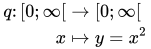
${\begin{aligned}q\colon [0;\infty {[}&\rightarrow [0;\infty {[}\\x&\mapsto y=x^{2}\end{aligned}}$

the (bijective) restriction of the square function to the set of non-negative real numbers. The inverse function of this function is called the square root function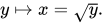 $y\mapsto x={\sqrt {y}}.$

Comments

Note that the square function explained by ${\mathbb {R}}\rightarrow {\mathbb {R}};x\mapsto x^{2}$ is defined for all real numbers but is not invertible. It is neither injective nor surjective.
The constraint of the square function is reversible and is inverted by the real root function. Since only non-negative real numbers occur as images of , the real root function is defined only for these numbers.
Due to the restriction of to non-negative real numbers made before the inversion, the values of the square root function are non-negative numbers. The restriction of the square function to other subsets of $\mathbb {R}$ in which different real numbers always have different squares would lead to other inverse functions, but these are not called real square root functions.

Examples

Square numbers and their square roots
Radikand	Square root	Radikand	Square root
1	1	121	11
4	2	144	12
9	3	169	13
16	4	196	14
25	5	225	15
36	6	256	16
49	7	289	17
64	8	324	18
81	9	361	19
100	10	400	20

The square root of a natural number is either an integer or irrational. The proof is analogous to Euclid's proof of the irrationality of the square root of 2.

Properties and calculation rules

The properties of the square root function result from the properties of the square function restricted to the set of non-negative real numbers:

${\sqrt {a\cdot b}}={\sqrt {a}}\cdot {\sqrt {b}}\;$ for $\;0\leq a,\,0\leq b$ .
${\sqrt {a\cdot b}}={\sqrt {-a}}\cdot {\sqrt {-b}}\;$ for $\;a\leq 0,\,b\leq 0$ .
$0\leq a<b\;\Longleftrightarrow \;0\leq {\sqrt {a}}<{\sqrt {b}}$ , i.e., the square root function is strictly monotonically increasing.
${\sqrt {a^{2}}}=|a|$ holds with the real magnitude for any real numbers .
On the other hand, $({\sqrt {a}})^{2}=a$ only valid for non-negative .
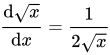The square root function is differentiable on $\mathbb{R} _{+}$ differentiable, there ${\frac {{\mathrm d}{\sqrt {x}}}{{\mathrm d}x}}={\frac {1}{2{\sqrt {x}}}}$ .
At the point 0 it is not differentiable, its graph has there a perpendicular tangent with the equation .
It is Riemann integrable on any closed subinterval its domain of definition, one of its primitive functions is $F(x)={\tfrac {2}{3}}\cdot {\sqrt {x^{3}}}$ .

Diagram of the square function (red and blue). By mirroring only the blue half on the bisector of the 1st quadrant, the diagram of the square root function (green) is created.

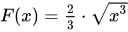Calculation of square roots from real numbers

Rational approximate values of some
square roots

${\begin{array}{ccccr}{\sqrt {2}}&\approx &{\sqrt {\frac {49}{25}}}&=&{\frac {7}{5}}\\{\sqrt {2}}&\approx &{\sqrt {\frac {289}{144}}}&=&{\frac {17}{12}}\\{\sqrt {2}}&\approx &{\sqrt {\frac {1681}{841}}}&=&{\frac {41}{29}}\\{\sqrt {3}}&\approx &{\sqrt {\frac {49}{16}}}&=&{\frac {7}{4}}\\{\sqrt {3}}&\approx &{\sqrt {\frac {361}{121}}}&=&{\frac {19}{11}}\\{\sqrt {5}}&\approx &{\sqrt {\frac {81}{16}}}&=&{\frac {9}{4}}\\{\sqrt {6}}&\approx &{\sqrt {\frac {2401}{400}}}&=&{\frac {49}{20}}\\{\sqrt {7}}&\approx &{\sqrt {\frac {64}{9}}}&=&{\frac {8}{3}}\\{\sqrt {8}}&\approx &{\sqrt {\frac {289}{36}}}&=&{\frac {17}{6}}\\{\sqrt {10}}&\approx &{\sqrt {\frac {361}{36}}}&=&{\frac {19}{6}}\\{\sqrt {11}}&\approx &{\sqrt {\frac {100}{9}}}&=&{\frac {10}{3}}\end{array}}$

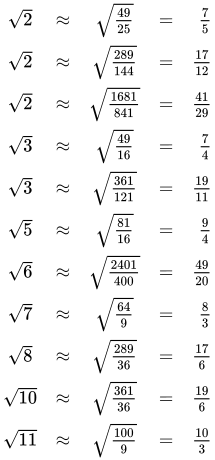
Even then, if the square root is to be taken from a natural number, the result is often an irrational number, whose decimal fraction is thus a non-periodic, non-breaking decimal fraction (namely, precisely when the result is not natural). The calculation of a square root that is not a rational number thus consists in determining an approximate value of sufficient accuracy. There are a number of ways to do this:

Written root extraction

This is an algorithm similar to the common method of written division.

Interval nesting

This procedure is quite easy to understand, although very tedious in practical implementation.

Example (approximate value for ${\sqrt {2}}$ ):

From $1^{2}=1<2$ = $2^{2}=4>2$ 2 {\displaystyle lies ${\sqrt {2}}$ and 2. Therefore, try $1{,}1^{2}$ , $1{,}2^{2}$ and so on. From $1{,}4^{2}=1{,}96<2$ 5 $1{,}5^{2}=2{,}25>2$ 2 {\displaystyle must lie ${\sqrt {2}}$ and 1,5. Continuing this procedure with more and more decimal places finally yields an approximate value with the desired accuracy:

$1{,}41421356^{2}<2<1{,}41421357^{2}\;\Rightarrow \;{\sqrt {2}}\approx 1{,}41421356$

Babylonian root extraction or Heron method

This iteration method is often used in programming the root calculation for calculators because it converges quickly. It is Newton's method for finding zeros applied to the function $x\mapsto x^{2}-a$ .

Taylor series development

The Taylor series development of the root function $t\mapsto {\sqrt {t}}$ with development place t=1 can be written as Taylor development of 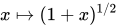$x\mapsto (1+x)^{1/2}$ around the place x=0 as binomial series

$\sum _{n=0}^{\infty }{\binom {1/2}{n}}\,x^{n}=\sum _{n=0}^{\infty }{\binom {2n}{n}}\,{\frac {(-1)^{n+1}}{(2n-1)\,4^{n}}}\,x^{n}=1+{\frac {1}{2}}x-{\frac {1}{8}}x^{2}+{\frac {1}{16}}x^{3}-{\frac {5}{128}}x^{4}\pm \dotsb$

can be found, because this series for converges $|x|\leq 1$ point-wise towards ${\sqrt {1+x}}$ With $x:=t-1$ this results in

${\sqrt {t}}=1+{\frac {1}{2}}(t-1)-{\frac {1}{8}}(t-1)^{2}+{\frac {1}{16}}(t-1)^{3}-{\frac {5}{128}}(t-1)^{4}\pm \dotsb$ for $0\leq t\leq 2.$

Calculation by means of CORDIC algorithm

This method is mainly used in arithmetic units, FPUs and microcontrollers.

Determining the square root graphically

One possibility is the cathetus theorem: The number whose square root is sought, is plotted on a number line from $0$ Over the distance between $0$ and a semicircle with radius $r={\tfrac {n}{2}}$ drawn (Thales circle). At a perpendicular to the base line is established which intersects the semicircle (height of a right triangle). The distance of this intersection to the zero point is the square root of (cathetus).

Square roots of complex numbers

If is a non-zero complex number, the equation has

$w^{2}=z$

exactly two solutions for which are also called roots or square roots of These lie in the Gaussian number plane on the two intersections of the circle around 0 with the radius ${\sqrt {|z|}}$ and the bisector of the angle between the $0$ rays starting from through respectively. The one of the two roots that lies in the right half-plane is called the principal value of the root. For negative (real) root with a positive imaginary part is the principal value.

If one writes the complex number in the form

$z=r\cdot {\rm {e^{\mathrm {i} \varphi },}}$

where φ $\varphi$ and are real with r>0 - π $-\pi <\varphi \leq \pi$ , then the following applies to the principal value of the root:

$w_{1}={\sqrt {r}}\cdot {\rm {e^{\mathrm {i} \varphi /2}}}$

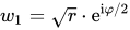
The second root value (the secondary value) is obtained by point mirroring (180° rotation) at the zero point:

$w_{2}={\sqrt {r}}\cdot {\rm {e^{\mathrm {i} (\varphi /2+\pi )}}}$

Definition

The complex function "square z", $q\colon {\mathbb {C}}\rightarrow {\mathbb {C}};z\mapsto z^{2}$ just like the real square function, has no inverse function because it is not injective, but unlike the real numbers it is surjective, that is, every complex number is the square of a complex number. One can therefore define complex square root functions analogously to the real (non-negative) square roots by restricting the domain of definition of to a subset of the complex numbers on which is injective and remains surjective. Depending on which subset one chooses for this, one obtains different branches of the square root function as an inverse.

The main branch of the complex square root function is obtained by taking as the domain of definition of

$D_{H}:=\{x+\mathrm {i} \,y\in \mathbb {C} \mid x>0{\text{ oder }}(x=0{\text{ und }}y\geq 0)\}$

this is the right half-plane of the complex number plane, from whose edge only the numbers with non-negative imaginary part $D_{H}$ belong to The restriction of to $D_{H}$ is a bijective mapping from $D_{H}$ to the complex numbers, hence its inverse function, the main branch of the square root on all of $\mathbb {C}$ defined. The value ${\sqrt {z}}$ this inverse function is called the principal value of the square root of . If by ${\sqrt {z}}$ a certain complex number is meant, then it is this principal value.

If given in Cartesian coordinates, i.e. $z=x+{\rm {iy}}$ with real numbers and then the result is

${\sqrt {z}}={\sqrt {x+{\rm {iy}}}}={\sqrt {\tfrac {|z|+x}{2}}}+\mathrm {i} \cdot \operatorname {sgn^{+}} (y)\cdot {\sqrt {\tfrac {|z|-x}{2}}}$

for the main value of the square root, where the function the value -1 $\operatorname {sgn^{+}}$ for negative and otherwise (i.e. also for y=0 and thus unlike the sign function $\operatorname{sgn}$ ) has the value 1:

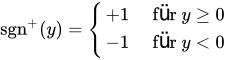
${\text{sgn}}^{+}(y)={\begin{cases}+1&{\text{ für }}y\geq 0\\-1&{\text{ für }}y<0\end{cases}}$

The only minor branch of is $-{\sqrt {z}}.$

Given in polar coordinates, 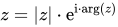$z=|z|\cdot {\mathrm e}^{{{\mathrm i}\cdot \arg(z)}}$ with $\arg(z)\in (-\pi ,\pi ]$ , then the principal value of the square root is given by

${\sqrt {z}}={\sqrt {|z|}}{\mathrm e}^{{{\mathrm i}\cdot \arg(z)/2}}$

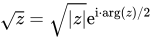
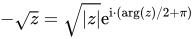where is ${\sqrt {|z|}}$ the real (non-negative) square root of |z| The minor value is again obtained as $-{\sqrt {z}}={\sqrt {|z|}}{\mathrm e}^{{{\mathrm i}\cdot (\arg(z)/2+\pi )}}$ .

The absolute value of the two roots is therefore the square root of the absolute value of the complex number. For the main value, the argument $\arg(z)$ ("the angle of z", see below) is halved. The other solution results geometrically from point mirroring of this principal value at the origin.

The argument of a complex number $z=x+{\mathrm i}\,y$ is the oriented angle $\angle (EOZ)$ in the complex number plane, the points are E(1|0), O(0|0) and Z(x|y) in real coordinates. In the picture of the following example, the argument of and the argument of marked in colour. w_1

· Complex square root

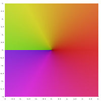
A branch of the square root

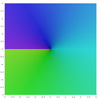
Second branch

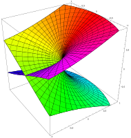
The Riemann area of the square root shows how the two branches merge.

Example: Calculation of a complex square root

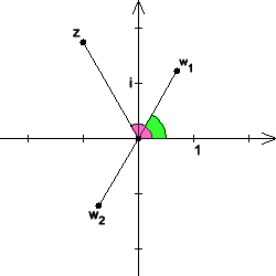
We are looking for the square roots of $z=-1+{\mathrm i}\,{\sqrt {3}}.$ First, the amount of the radicand is determined:

$|z|=\left|-1+{\mathrm i}{\sqrt {3}}\right|={\sqrt {(-1)^{2}+({\sqrt {3}})^{2}}}={\sqrt {1+3}}={\sqrt {4}}=2$

This gives the main value of the square root as

${\begin{aligned}w_{1}&={\sqrt {\tfrac {2+(-1)}{2}}}+\mathrm {i} \cdot \operatorname {sgn^{+}} ({\sqrt {3}})\cdot {\sqrt {\tfrac {2-(-1)}{2}}}\\[0.3em]&={\sqrt {\tfrac {1}{2}}}+\mathrm {i} \cdot (+1)\cdot {\sqrt {\tfrac {3}{2}}}={\sqrt {2}}\cdot \left({\tfrac {1}{2}}+\mathrm {i} \cdot {\tfrac {1}{2}}{\sqrt {3}}\right)\end{aligned}}$

The other root is obtained by reversing the sign:

$w_{2}=-w_{1}={\sqrt {2}}\cdot \left(-{\tfrac {1}{2}}-{\mathrm i}\cdot {\tfrac {1}{2}}{\sqrt {3}}\right)$

Power law

The power law

$(a\cdot b)^{r}=a^{r}\cdot b^{r}\qquad \qquad \qquad \qquad \qquad \qquad \quad {\text{(P)}}$

does not hold for $r=1/2$ for all $a,b\in \mathbb {C}$ even for the principal values of the roots.
This can already be seen from the special case resulting from the
further specification $a=b=:z$

${\sqrt {z^{2}}}=\left({\sqrt {z}}\right)^{2},$

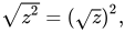
which, because of the identity $\left({\sqrt {z}}\right)^{2}=z$ becomes

${\sqrt {z^{2}}}=z$

according to which every negative number obviously already provides a counterexample, for example $z=-1$ :

Because $(-1)^{2}=1$ and $\arg(1)=0$ the principal value of ${\sqrt {(-1)^{2}}}$ has the argument $\arg({\sqrt {1}})=0/2=0$ while the principal value of 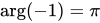$\arg(-1)=\pi$ has the argument

Comments

Since principal values of roots from positive radicands must be positive, the counterexample shows that there cannot be a square root function for which the power law ${\text{(P)}}$ all $a,b\in \mathbb {C}$ , cannot exist.
For $r=1/2$ and any one can $a,b\in \mathbb {C}$ freely choose the "sign" of two of the three roots in ${\text{(P)}}$ after which exactly one possibility remains for the "sign" of the last third.

Square roots modulo n

Also in the residue class ring ${\mathbb {Z}}/n{\mathbb {Z}}$ can be defined as square roots. Quite analogously to the real and complex numbers, is called a square root of holds:

$q^{2}\equiv x{\bmod {n}}$

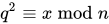
However, to calculate square roots modulo must use different methods than when calculating real or complex square roots. To determine the square roots of modulo , one can proceed as follows:

First determine the prime factorisation

$n=p_{1}^{{m_{1}}}\cdot p_{2}^{{m_{2}}}\dotsm p_{{k}}^{{m_{k}}}$

of the modulus and then the solutions modulo the individual prime powers $p^{m}$ . Finally, these solutions are put together using the Chinese Remainder Theorem to find the solution.

Calculation of square roots modulo a prime number p

The case p=2 is simple: Because 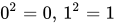$0^{2}=0,\,1^{2}=1$ and $1\not \equiv 0{\bmod {2}}$ modulo 2 every number has a uniquely determined square root, namely itself. For prime numbers not equal to 2, the calculation of the square roots of done like this:

To test whether a square root in ${\mathbb Z}/p{\mathbb Z}$ , calculate the value of the Legendre symbol

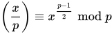$\left({\frac {x}{p}}\right)\equiv x^{\frac {p-1}{2}}{\bmod {p}}$ ,

because it is valid:

$\left({\frac {x}{p}}\right)={\begin{cases}-1,&{\text{wenn }}x{\text{ quadratischer Nichtrest modulo }}p{\text{ ist}}\\0,&{\text{wenn }}x{\text{ und }}p{\text{ nicht teilerfremd sind }}\\1,&{\text{wenn }}x{\text{ ein quadratischer Rest modulo }}p{\text{ ist}}\end{cases}}$

In the first case has no square root in ${\mathbb Z}/p{\mathbb Z}$ and in the second case only the square root 0. So the interesting case is the third case and therefore we assume in the following that ${\bigl (}{\tfrac {x}{p}}{\bigr )}=1$ holds.

Calculation for the case p mod 4 = 3

If the Legendre symbol ${\bigl (}{\tfrac {x}{p}}{\bigr )}$ is equal to 1, then

$q\equiv \pm x^{\frac {p+1}{4}}{\bmod {p}}$

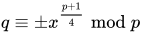
the two square roots of modulo .

Calculation for the case p mod 4 = 1

If the Legendre symbol ${\bigl (}{\tfrac {x}{p}}{\bigr )}$ is equal to 1, then

$q\equiv \pm {\frac {x}{2r}}\left(W_{\frac {p-1}{4}}+W_{\frac {p+3}{4}}\right){\bmod {p}}$

the two square roots of modulo . Here one chooses that

$\left({\frac {r^{2}-4x}{p}}\right)=-1$

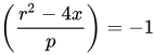
is valid. To do this, one can simply test different values of The sequence $W_{n}$ is recursive through

$W_{n}={\begin{cases}r^{2}/x-2,&{\text{ wenn }}n=1\\W_{{n/2}}^{2}-2,&{\text{ wenn }}n{\text{ gerade}}\\W_{{(n+1)/2}}W_{{(n-1)/2}}-W_{1},&{\text{ wenn }}n>1{\text{ ungerade}}\end{cases}}$

defined.

Calculation example for x=3 and p=37 :

According to the above formula, the square roots of are given by

$q\equiv \pm {\frac {x}{2r}}\left(W_{9}+W_{10}\right){\bmod {3}}7$

given. For one finds by trial and error the value r = 2 because it holds:

$\left({\frac {r^{2}-4x}{p}}\right)\equiv (r^{2}-4x)^{\frac {p-1}{2}}\equiv (-8)^{18}\equiv 36\equiv -1{\bmod {3}}7$

values for $W_{9}$ and $W_{{10}}$ result like this:

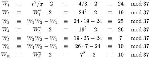
${\begin{matrix}W_{1}&\equiv &r^{2}/x-2&\equiv &4/3-2&\equiv &24&{\bmod {3}}7\\W_{2}&\equiv &W_{1}^{2}-2&\equiv &24^{2}-2&\equiv &19&{\bmod {3}}7\\W_{3}&\equiv &W_{1}W_{2}-W_{1}&\equiv &24\cdot 19-24&\equiv &25&{\bmod {3}}7\\W_{4}&\equiv &W_{2}^{2}-2&\equiv &19^{2}-2&\equiv &26&{\bmod {3}}7\\W_{5}&\equiv &W_{2}W_{3}-W_{1}&\equiv &19\cdot 25-24&\equiv &7&{\bmod {3}}7\\W_{9}&\equiv &W_{4}W_{5}-W_{1}&\equiv &26\cdot 7-24&\equiv &10&{\bmod {3}}7\\W_{10}&\equiv &W_{5}^{2}-2&\equiv &7^{2}-2&\equiv &10&{\bmod {3}}7\\\end{matrix}}$

Inserting these values gives

$q\equiv \pm {\frac {x}{2r}}\left(W_{9}+W_{10}\right)\equiv \pm {\frac {3}{4}}(10+10)\equiv \pm 15{\bmod {3}}7.$

That is: 15 and 22 are the two square roots of 3 modulo 37.

Square roots of matrices

→ Main article: Square root of a matrix

The root of a square matrix is all matrices which, when multiplied by themselves, give

$A=B\cdot B\Leftrightarrow B{\text{ ist Wurzel von }}A$

As with the root of real or complex numbers, the root of matrices is not necessarily unique. However, if we consider only positive definite symmetrical matrices, the root formation is unambiguous: every positive definite symmetrical matrix has a unambiguous positive definite symmetrical root $A^{{\frac {1}{2}}}.$ It is obtained by diagonalising using an orthogonal matrix (this is always possible according to the spectral theorem) and then replacing the diagonal elements with their roots; however, the positive root must always be chosen. See also Cholesky decomposition. The uniqueness follows from the fact that the exponential mapping is a diffeomorphism from the vector space of symmetric matrices onto the subset of positive definite symmetric matrices.

Square root of an approximated integral operator

One can take the definite integral function 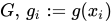$G,\,g_{i}:=g(x_{i})$ from 0 to $x_{i}$ with $x_{i}=i\Delta x$ and $i=0,1,\dotsc ,n-1$ a given function which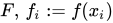 $F,\,f_{i}:=f(x_{i})$ $f_{i}$ assumes the values at the equidistant grid points $x_{i}$ as a matrix multiplication G=FI as follows (for n=4 ):

$G=FI={\begin{pmatrix}g_{0}&g_{1}&g_{2}&g_{3}\\0&g_{0}&g_{1}&g_{2}\\0&0&g_{0}&g_{1}\\0&0&0&g_{0}\end{pmatrix}}={\begin{pmatrix}f_{0}&f_{1}&f_{2}&f_{3}\\0&f_{0}&f_{1}&f_{2}\\0&0&f_{0}&f_{1}\\0&0&0&f_{0}\end{pmatrix}}{\begin{pmatrix}\Delta x&\Delta x&\Delta x&\Delta x\\0&\Delta x&\Delta x&\Delta x\\0&0&\Delta x&\Delta x\\0&0&0&\Delta x\end{pmatrix}}$

It is vividly clear that one can repeat this operation and thus $H,\,h_{i}:=h(x_{i})$ obtain the double integral

$H=GI=FII=FI^{2}$

Thus, the matrix can be understood as a numerically approximated integral operator.

The matrix is not diagonalisable and its Jordanian normal form is:

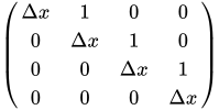
${\begin{pmatrix}\Delta x&1&0&0\\0&\Delta x&1&0\\0&0&\Delta x&1\\0&0&0&\Delta x\end{pmatrix}}$

To draw a square root from this, one could proceed as described for the non-diagonalisable matrices. However, there is a more direct formal solution in this case as follows:

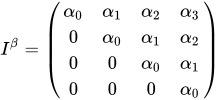
$I^{\beta }={\begin{pmatrix}\alpha _{0}&\alpha _{1}&\alpha _{2}&\alpha _{3}\\0&\alpha _{0}&\alpha _{1}&\alpha _{2}\\0&0&\alpha _{0}&\alpha _{1}\\0&0&0&\alpha _{0}\end{pmatrix}}$

with α 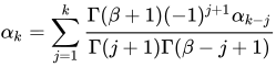$\alpha _{0}=(\Delta x)^{\beta }$ , $\alpha _{k}=\sum _{{j=1}}^{{k}}{\frac {\Gamma (\beta +1)(-1)^{{j+1}}\alpha _{{k-j}}}{\Gamma (j+1)\Gamma (\beta -j+1)}}$ and $k=1,2,\dotsc ,n-1$ .

In it, the indices of α $\alpha$ denote the subdiagonals (0 is the diagonal) and the exponent β $\beta$ is equal to ${\tfrac {1}{2}}$ . If Δ $\Delta x$ assumed to be real and positive, then $(\Delta x)^{{\frac {1}{2}}}$ real and positive by definition.

Thus, one can numerically approximate a "half" definite integral 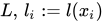$L,\,l_{i}:=l(x_{i})$ from 0 to $x_{i}$ the function f(x) as follows:

$L=FI^{\beta }={\begin{pmatrix}l_{0}&l_{1}&l_{2}&l_{3}\\0&l_{0}&l_{1}&l_{2}\\0&0&l_{0}&l_{1}\\0&0&0&l_{0}\end{pmatrix}}={\begin{pmatrix}f_{0}&f_{1}&f_{2}&f_{3}\\0&f_{0}&f_{1}&f_{2}\\0&0&f_{0}&f_{1}\\0&0&0&f_{0}\end{pmatrix}}{\begin{pmatrix}\alpha _{0}&\alpha _{1}&\alpha _{2}&\alpha _{3}\\0&\alpha _{0}&\alpha _{1}&\alpha _{2}\\0&0&\alpha _{0}&\alpha _{1}\\0&0&0&\alpha _{0}\end{pmatrix}}$

If one looks for all operators which, multiplied by themselves, give the approximated integral operator , one must also insert the negative sign, that is, there are two solutions $\pm I^{{\frac {1}{2}}}$ .

To derive the formula, one can first invert , $\beta$ exponentiate the result with β and finally invert again.

Author

AlegsaOnline.com Square root Leandro Alegsa

URL: https://en.alegsaonline.com/art/92938

How to cite this article

APA

Alegsa, L. (May 6, 2026). Square root. AlegsaOnline.com. https://en.alegsaonline.com/art/92938

MLA

Alegsa, Leandro. “Square root.” AlegsaOnline.com, May 6, 2026, https://en.alegsaonline.com/art/92938

Chicago

Alegsa, Leandro. “Square root.” AlegsaOnline.com. Updated May 6, 2026. https://en.alegsaonline.com/art/92938

BibTeX

@misc{alegsaonline_92938,
  author = {Alegsa, Leandro},
  title = {Square root},
  year = {2026},
  howpublished = {AlegsaOnline.com},
  url = {https://en.alegsaonline.com/art/92938},
  note = {Updated: May 6, 2026; Language: en}
}

TXT

Leandro Alegsa. “Square root.” AlegsaOnline.com. Updated: May 6, 2026. https://en.alegsaonline.com/art/92938

Overview and definition

Image gallery

Basic properties and distinctions

Real versus complex square roots

Notable examples and irrationality

Computation methods

History and applications

Examples, identities and cautions

Preliminary remark on the definitions

Square roots of real numbers

Comments

Examples

Properties and calculation rules

Calculation of square roots from real numbers

Determining the square root graphically

Square roots of complex numbers

Definition

Example: Calculation of a complex square root

Power law

Square roots modulo n

Calculation of square roots modulo a prime number p

Calculation for the case p mod 4 = 3

Calculation for the case p mod 4 = 1

Square roots of matrices

Square root of an approximated integral operator

See also

Related articles

Author

Share