
Skew lines (nonparallel, nonintersecting lines in 3D geometry)
Lines in three-dimensional space that neither intersect nor are parallel; defined by noncoplanarity. Article covers definition, algebraic tests, distance formula, examples and applications.
Overview
Skew lines are straight lines in space that do not meet and are not parallel. Unlike two lines in a single plane, which either intersect or are parallel, skew lines exist only in three or more dimensions: they lie in different planes and therefore cannot be placed on one common plane without moving them.
Image gallery
2 Images

Characteristics and algebraic test
In analytic geometry each line can be written in parametric vector form: L1: r = p + t u and L2: r = q + s v, where p and q are position vectors of points on the lines and u and v are their direction vectors. The two necessary conditions for skewness are:
- u and v are not parallel (equivalently u × v ≠ 0), and
- the vector connecting a point on one line to a point on the other, w = q − p, is not coplanar with u and v. Algebraically this means the scalar triple product w · (u × v) ≠ 0.
If u and v were parallel and w · (u × v) = 0, the lines would be parallel or coincident; if u × v ≠ 0 but w · (u × v) = 0, the lines lie in a common plane and so intersect.
Distance and shortest segment
Two skew lines have a unique shortest segment that is perpendicular to both lines. The length of this segment equals the distance between the lines and can be computed by | (q − p) · (u × v) | / |u × v|. This formula uses the magnitude of the cross product of direction vectors and the scalar triple product, giving a coordinate-free measure of separation.
Examples and applications
Classic geometric examples are opposite edges of a rectangular box or a cube: those edges neither meet nor remain parallel. Skew lines appear in mechanical design, computer graphics, collision detection, robotics and CAD, where spatial relationships between components must be analyzed in three dimensions.
Distinctions and practical notes
Do not confuse skew lines with parallel lines (same direction, never meet) or with intersecting lines (share a point). Determining whether two 3D lines intersect can be done by solving their parametric equations; if no common (s,t) exists and the lines are not parallel, they are skew. These criteria and formulas are widely used in analytic and computational geometry.


Calculation of the distance between two skew lines
The uniquely determined path of smallest length  connecting two skew lines
  and called the common perpendicular of the two lines. The line on which the common perpendicular lies is called the minimum transversal of the two lines. This is the uniquely determined straight line which is at right angles to the two straight lines. The length of the common perpendicular of and is the distance
  of the two straight lines.
Given the skew lines and with the supporting points  and
and  resp. the support vectors
 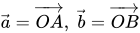 and the direction vectors
  and
and  . Then the parameter forms of the linear equations are
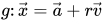
 ,
,
Where 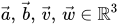 holds and the three vectors
  must be linearly independent.
The normal vector  which is perpendicular to the two direction and can be calculated via the cross product:
 and bring to length 1:
 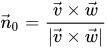 .
.
The calculation of the distance is possible by the orthogonal projection of the connection vector of the support points on the normal vector. To do this, the normal vector is brought to the length 1. The distance of the two skew lines is then
 .
.
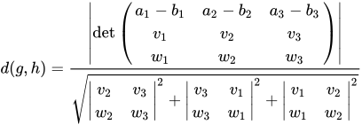
Notation with determinants
The two straight line equations are written out as follows
![{\displaystyle g\colon {\vec {x}}=\left({\begin{smallmatrix}a_{1}\\[0.7ex]a_{2}\\[0.7ex]a_{3}\end{smallmatrix}}\right)+r\left({\begin{smallmatrix}v_{1}\\[0.7ex]v_{2}\\[0.7ex]v_{3}\end{smallmatrix}}\right)}](https://www.alegsaonline.com/image/f3160bfc87366a2eac81e4665f233f44189958a4.svg)
![{\displaystyle h\colon {\vec {x}}=\left({\begin{smallmatrix}b_{1}\\[0.7ex]b_{2}\\[0.7ex]b_{3}\end{smallmatrix}}\right)+s\left({\begin{smallmatrix}w_{1}\\[0.7ex]w_{2}\\[0.7ex]w_{3}\end{smallmatrix}}\right)\ \ \,r,s\in \mathbb {R} }](https://www.alegsaonline.com/image/e993c87603d44aa990413dee0130fdc4c25de39e.svg) .
.
The distance between the two skew lines using the determinant det is then
 .
.

Determination of the perpendicular points
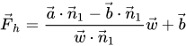
The perpendicular foot point  is obtained by setting up an auxiliary plane
  point lies on the auxiliary plane, and span the auxiliary plane.
 ,
,
where the normal vector is determined by
.
The intersection of and gives the plumb bob :
 where
where 
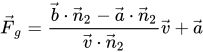
Similarly, we obtain  with the plane
  and its intersection with :
 where
where 
With this method, the distance  not need to be calculated.
The perpendicular foot points can also be determined by setting the two (for the time being unknown) points:
 and
and 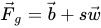
and then move one along and make it coincide with the other:
 .
.
A line-by-line resolution yields a system with three variables:  ,
,  and
and  . The footers are then:
 and
and  .
.
The distance given by 

Related articles
Author
AlegsaOnline.com Skew lines (nonparallel, nonintersecting lines in 3D geometry) Leandro Alegsa
URL: https://en.alegsaonline.com/art/90906