
Riemann sum — approximation of definite integrals
A Riemann sum approximates a definite integral by summing products of function values and interval widths; it underlies the Riemann integral and many numerical integration methods.
Overview
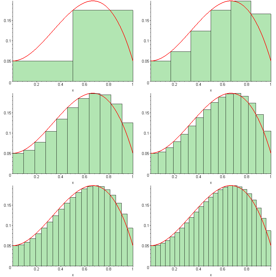
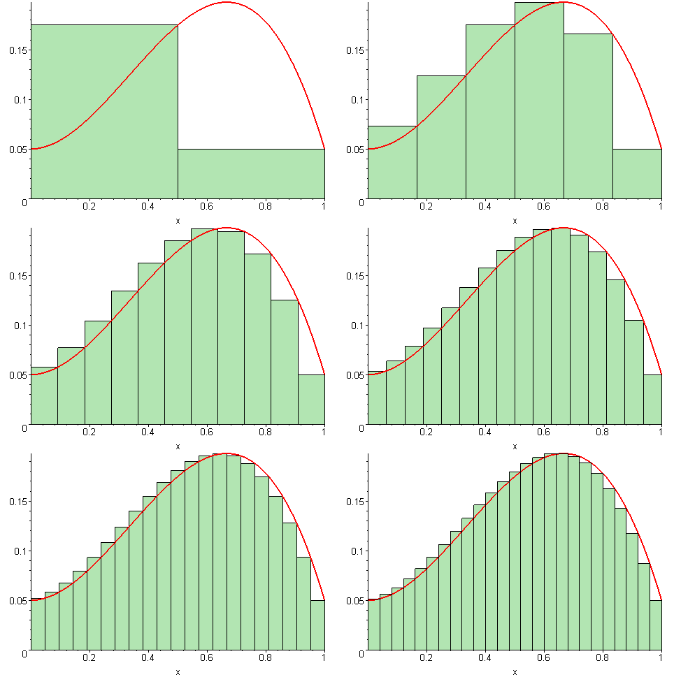
In mathematics, a Riemann sum is a simple and widely used method for approximating the definite integral of a function over a given interval. Geometrically, the definite integral is often interpreted as the area under a curve, and a Riemann sum replaces that region by a finite collection of elementary shapes whose areas are easy to compute. As the pieces become smaller and more numerous, the sum typically approaches the true integral.
Image gallery
5 Images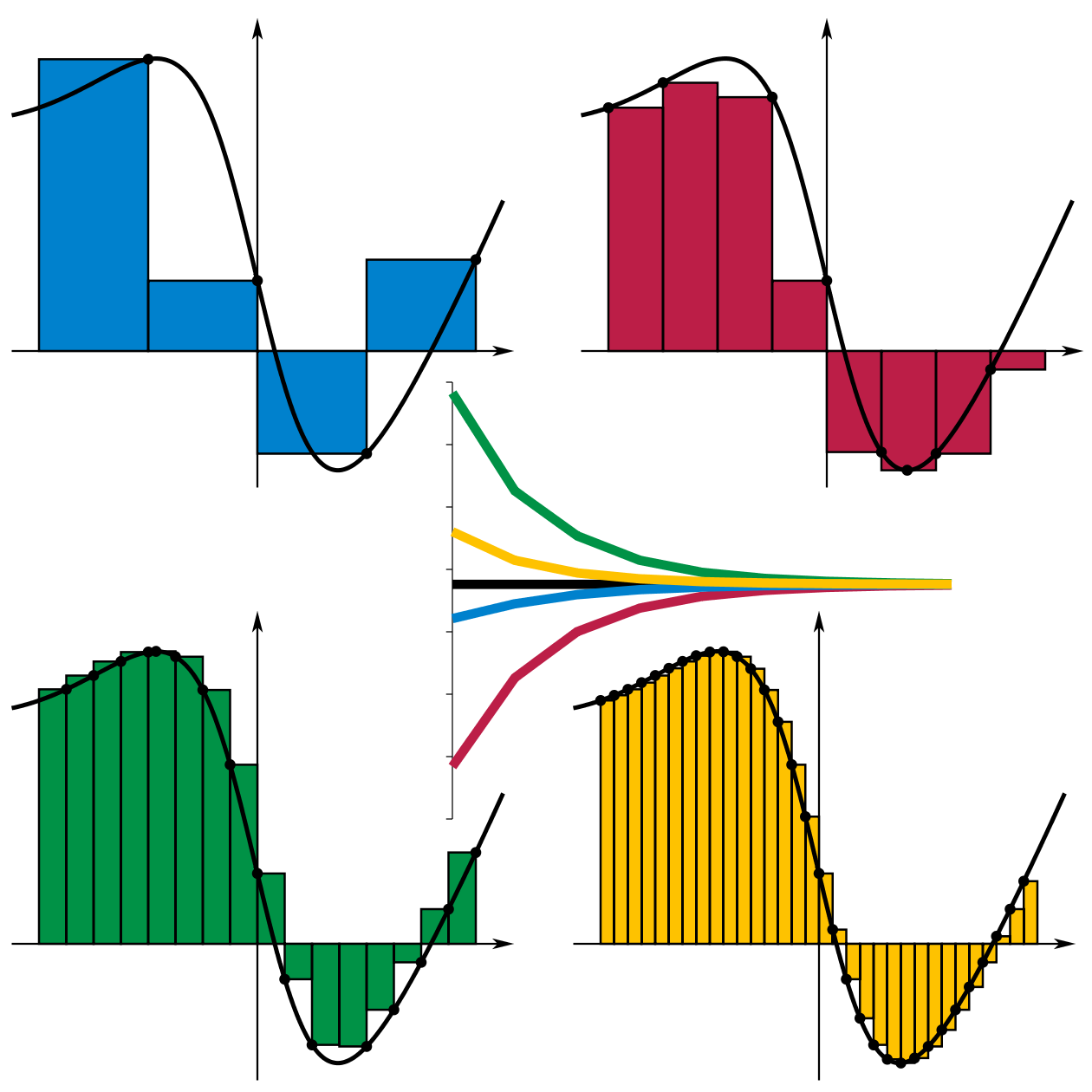


Formal idea and construction
To form a Riemann sum one chooses a partition of the interval into subintervals, selects a sample point in each subinterval, evaluates the function at those points, multiplies each function value by the subinterval width, and adds the results. If the interval [a,b] is split into n subintervals with widths Δx_i and sample points x*_i, the Riemann sum is the finite sum Σ f(x*_i) Δx_i. The key parameter is the mesh (or norm) of the partition: the length of the largest subinterval. If the mesh tends to zero and the sums converge to a limit, that limit is the Riemann integral of the function over [a,b].
Common choices and practical types
Different choices of sample points and shapes give familiar variants and affect accuracy and computational effort. Simple variants include:
- Left Riemann sum: use the left endpoint of each subinterval (sometimes linked to rectangles).
- Right Riemann sum: use the right endpoint.
- Midpoint rule: use the midpoint of each subinterval; often more accurate than endpoints for the same partition.
- Improved rules: the trapezoidal rule (using trapezoids) and Simpson's rule (approximating with parabolas) fit higher-degree shapes to increase accuracy.
Convergence and error
Because the simple shapes rarely match the original region exactly, a Riemann sum differs from the true integral by an error. Error estimates depend on the function's smoothness and on the rule used: for example, the midpoint and trapezoidal rules have errors that decrease proportionally to the square of the mesh under moderate smoothness assumptions, while Simpson's rule typically decreases faster. Reducing the mesh size—making subintervals smaller—reduces error; in the limit as the mesh goes to zero, sums that converge define the Riemann integral. The limiting process provides both a computational tool and a foundational definition of integration.
Uses, examples and importance
Riemann sums are practical for hand calculations, computer algorithms, and as a conceptual bridge between discrete sums and continuous integrals. A simple illustrative example is f(x)=x on [0,1]. Using n equal subintervals and right endpoints gives the sum (1/n)·(1/n + 2/n + ... + n/n) which simplifies to (n+1)/(2n) and tends to 1/2 as n→∞, matching the exact integral. In numerical analysis, Riemann-sum-based rules form the basis of quadrature methods and are used when an antiderivative is difficult to obtain analytically.
History and distinctions
The concept is named after the 19th-century mathematician Bernhard Riemann, who clarified integration by formalizing limits of sums of this type; the finite sums themselves had been used earlier in various forms. The Riemann integral is intuitive and sufficient for many applications, but it is not the most general notion of integral. Modern measure theory introduces the Lebesgue integral, which can integrate a wider class of functions and handles limiting processes differently, although for many functions both integrals coincide.
Related topics and further reading
For deeper study, one examines partitions and refinement, rigorous definitions of mesh and limit, and proofs of convergence for continuous functions. Connections to series, improper integrals, and numerical quadrature methods extend the basic idea. Introductory textbooks and online resources provide worked examples and error bounds; see introductory pages on basic integration techniques and numerical integration for practical algorithms and code examples. Additional resources: Riemann sum and its variants, definite integrals, and standard texts on analysis and numerical methods available through educational repositories (function theory, areas and geometry, polynomial approximation, rectangular rules, trapezoidal corrections, and error analysis).
For interactive demonstrations and step-by-step computations that build intuition, consult teaching materials and visualization tools that illustrate how sums of simple shapes converge to continuous area as partitions become finer. Reliable introductory expositions and lecture notes can be sought via educational portals and university course pages referenced in mathematical curricula (mathematics overview, function properties, biographical notes).
Questions and answers
Q: What is a Riemann sum?
A: The Riemann sum is a method of approximating the integral of a function over an interval, often used when finding the closed form integral is difficult or impossible.
Q: How is the Riemann sum calculated?
A: The Riemann sum is calculated by splitting the region into equal parts and replacing the function in each part with a shape such as rectangles, trapezoids, parabolas, or cubics. The area of the similar shape can then be calculated.
Q: What is the purpose of using shapes in the Riemann sum?
A: Using shapes in the Riemann sum helps to approximate the area under a curve in a graph and to calculate the integral of a function over an interval.
Q: Do different shapes used in Riemann sum affect the accuracy of the approximation?
A: Yes, the shapes used in Riemann sum influence how accurate the approximation is. More complex shapes give a higher accuracy, but this also means that calculating the approximation becomes more difficult.
Q: Can Riemann sum be used to define integration?
A: Yes, the Riemann sum may also be used to define the integration operation.
Q: Who is Bernhard Riemann?
A: Bernhard Riemann was a German mathematician after whom the Riemann sum is named.
Q: What can be done to reduce the error in the Riemann sum?
A: The error in the Riemann sum can be reduced by dividing up the region more finely, using smaller and smaller shapes. As the shapes get smaller and smaller, the sum approaches the Riemann integral.
Related articles
Author
AlegsaOnline.com Riemann sum — approximation of definite integrals Leandro Alegsa
URL: https://en.alegsaonline.com/art/82856