Percentile (statistics) — definition, calculation, uses, and distinctions
Definition and explanation of percentiles: how they are computed, common methods, historical notes, uses in testing and growth charts, and differences from related measures.
A percentile (also called a centile) is a statistical measure that indicates the relative standing of a value within a collection of observations. Saying that a score is at the 30th percentile means that about 30% of values in the reference group are equal to or below that score. Percentiles partition ordered data into 100 equal parts and give a simple way to express how unusual or typical a particular observation is compared with the rest of a data set.
Image gallery
3 Images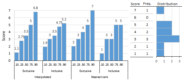

Basic meaning and notation
Percentiles are indexed from 0 to 100. The 0th percentile is at the minimum of the sample and the 100th percentile at the maximum. Commonly cited values include the 25th, 50th and 75th percentiles, often called the first, second and third quartiles; the 50th percentile is also the median. In practice, percentiles describe a cutoff value: the pth percentile is a value below which approximately p percent of the observations fall.
How percentiles are computed
Computing a percentile requires ordering the observations from smallest to largest and locating the position associated with the desired percentage. For discrete samples the position may not be an integer, and several conventions exist to resolve this. Two widely used approaches are:
- Nearest-rank (or empirical) method: take the element whose rank corresponds to p percent of the sample size. This is simple and common in educational reporting.
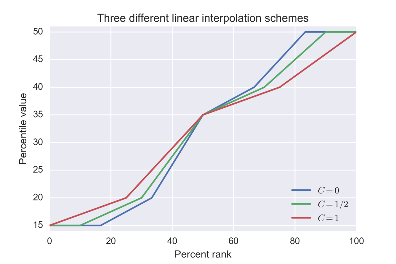
- Interpolation methods: estimate a value between neighboring observations when the computed rank is fractional. Many statistical packages use variants of linear interpolation to produce smooth quantiles.
Because multiple definitions exist, published percentile values may differ slightly depending on the chosen algorithm; this matters most for small samples.
History and context
The idea of dividing distributions into equal-probability parts dates back to early work on descriptive statistics and probability in the 19th and early 20th centuries. The term "percentile" follows naturally from the practice of using percent divisions. Percentiles gained practical importance with standardized testing and growth charts, where they provide an immediately understandable scale for relative performance or development.
Uses, examples and interpretation
Percentiles are widely used because they are intuitive and robust to extreme values. Typical applications include:
- Educational testing — reporting how a student's score compares with peers (percentile rank).
- Medical growth charts — indicating how a child's height or weight compares with a reference population.
- Income and epidemiology studies — describing inequality or risk by showing the fraction of the population below given thresholds.
Interpretation must be cautious: being in a high percentile does not convey the magnitude of difference from other scores, only the relative position. Percentiles are not the same as percentages of a maximum possible score, nor do they measure central tendency by themselves.
Related measures and notable facts
Percentiles are one type of quantile; other related concepts include quartiles, deciles (ten equally sized groups), and percent ranks (the percentage of observations at or below a value). Compared with means or variances, percentiles are less sensitive to outliers and are useful for summarizing skewed distributions. For rigorous work it is important to state the computational method used and whether percentiles refer to a sample or to a theoretical population distribution. For further introductory material see general statistics references.
Definition
Let ⌊  denote the rounding function. It rounds each number
  to the nearest smaller integer. For example, ⌊
  and ⌊
and ⌊  .
.
Given a sample  size
size  , whose elements are ordered by size. This means that
 .
.
Then, for a number 

the empirical  -quantile of
  .
.
Some definitions exist that differ from the definition given here.
Example
The following sample consists of ten random integers (drawn from the numbers between zero and one hundred, fitted with the discrete uniform distribution):

Sort provides the sample
 .
.
It is  .
.
For  we get
  . Since this is an integer, we obtain via the definition

For  we get
  . The rounding function then yields ⌊
  and thus
 .
.
Similarly, for  directly obtain
  and thus ⌊
  , so
, so
 .
.
In contrast to the arithmetic mean, the empirical quantile is robust to outliers. This means that if values of a sample above (or below) a certain quantile are replaced by a value above (or below) the quantile, the quantile itself does not change. This is based on the fact that quantiles are determined only by their order and thus their position with respect to each other, and not by the concrete numerical values of the sample. Thus, in the case of the sample above, the arithmetic mean would be  . However, if we now modify the largest value of the sample, we set for example
 ,
,
so  , whereas the median, lower quartile, and upper quartile remain unchanged because the order of the sample has not changed.
Special quantiles
For certain values, the associated quantiles have proper names. They are briefly introduced in the following. It should be noted that the corresponding quantiles of probability distributions are also partly designated with the same proper names.
Median
→ Main article: Median
The median is the  quantile and thus divides the sample into two halves: one half is smaller than the median, the other larger than the median. Together with the mode and the arithmetic mean, it is an important location parameter in descriptive statistics.
Terzil
The two -quantiles for  and
and  called terciles. They divide the sample into three equal parts: one part is smaller than the lower tercile (= {\tfrac
  -quantile), one part is larger than the upper tercile (=
  -quantile), and one part lies between the terciles.
Quartile
The two quantiles with and called quartiles. Here, the  quantile is called the lower quartile and the
  quantile is called the upper quartile. Half of the sample lies between the upper and lower quartiles, and a quarter of the sample lies below the lower quartile and above the upper quartile, respectively. The interquartile range, a measure of dispersion, is defined on the basis of the quartiles.
Quintile
Quintiles are the four quantiles with  Accordingly, 20% of the sample is below the first quintile and 80% above it, 40% of the sample is below the second quintile and 60% above it, and so on.
Decile
The quantiles for multiples of  , i.e. for
  are called deciles. Here, the quantile is called the first decile, the
  quantile is called the second decile, etc. Below the first decile are 10% of the sample, above correspondingly 90% of the sample. Similarly, 40% of the sample lies below the fourth decile and 60% above.
Percentile
Percentiles are the quantiles from  to
to  in steps of .
Derived terms
From the quantiles, certain measures of dispersion can be derived. The most important is the interquartile range.
 .
.
It indicates how far apart the upper and lower quartiles are and thus how wide the range is in which the middle 50% of the sample lies. Somewhat more generally, the (inter)quantile distance can be defined as  for
for  . It indicates how wide is the range in which the mean
  the sample lies. For it corresponds to the interquartile range.
Another derived measure of dispersion is the mean absolute deviation from the median.
View
One way of displaying quantiles is the box plot. Here, the entire sample is represented by a box - provided with two antennas. The outer boundaries of the box are the upper and lower quartiles. Thus, half of the sample is in the box. The box itself is subdivided again, the subdividing line is the median of the sample. The antennas are not uniformly defined. One possibility is to choose the first and the ninth decile as the limits of the antennas.

Related articles
Author
AlegsaOnline.com Percentile (statistics) — definition, calculation, uses, and distinctions Leandro Alegsa
URL: https://en.alegsaonline.com/art/75746