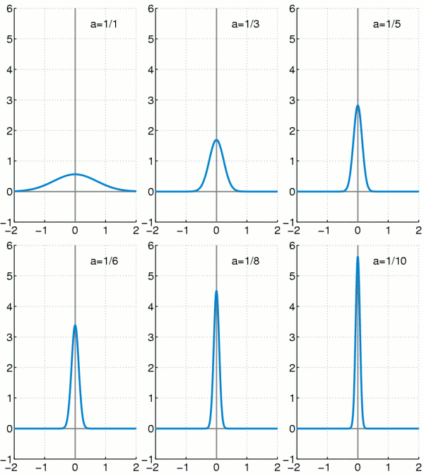
Normal distribution

The normal or Gaussian distribution (after Carl Friedrich Gauss) is an important type of continuous probability distribution in stochastics. Its probability density function is also called Gaussian function, Gaussian normal distribution, Gaussian distribution curve, Gaussian curve, Gaussian bell curve, Gaussian bell function, Gaussian bell or simply bell curve.

The special significance of the normal distribution is based, among other things, on the central limit theorem, according to which distributions that result from additive superposition of a large number of independent influences are approximately normally distributed under weak conditions. The family of normal distributions forms a location-scale family.

The deviations of the measured values of many natural, economic and engineering processes from the expected value can be described by the normal distribution (often logarithmic normal distribution for biological processes) in a very good approximation (especially processes that act in several factors independently in different directions).

Random variables with normal distribution are used to describe random processes such as:

random scattering of measured values,
random deviations from the nominal dimension during the production of workpieces,
Description of Brownian molecular motion.

In actuarial science, the normal distribution is suitable for modeling loss data in the range of medium loss amounts.

In measurement technology, a normal distribution is often used to describe the scatter of measured values.

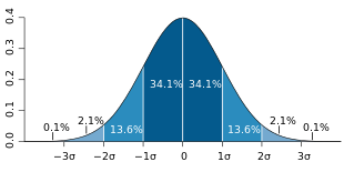
The standard deviation σ $\sigma$ describes the width of the normal distribution. The half-width of a normal distribution is approximately $2{,}4$ times (exactly $2{\sqrt {2\ln 2}}$ ) the standard deviation. It holds approximately:

In the interval of deviation $\pm \sigma$ from the expected value 68.27 % of all measured values are found,
In the interval of deviation $\pm 2\sigma$ from the expected value 95.45 % of all measured values can be found,
In the interval of deviation $\pm 3\sigma$ from the expected value 99.73 % of all measured values can be found.

And, conversely, the maximum deviations from the expected value can be found for given probabilities:

50% of all measured values have a deviation of at most $0{,}675\sigma$ from the expected value,
90% of all measured values have a deviation of at most $1{,}645\sigma$ from the expected value,
95% of all measured values have a deviation of at most $1{,}960\sigma$ from the expected value,
99% of all measured values have a deviation of at most $2{,}576\sigma$ from the expected value.

Thus, in addition to the expected value, which can be interpreted as the center of gravity of the distribution, the standard deviation can also be assigned a simple meaning with respect to the magnitudes of the occurring probabilities or frequencies.

Definition

A continuous random variable has a (Gaussian or) normal distribution with expected value μ $\mu$ and variance σ $\sigma ^{2}$ ( $-\infty <\mu <\infty ,\sigma ^{2}>0$ ), often written as $X\sim {\mathcal {N}}\left(\mu ,\sigma ^{2}\right)$ , if has the following probability density:

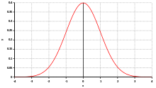
The graph of this density function has a "bell shape" and is symmetric with the parameter μ $\mu$ as the center of symmetry, which also represents the expected value, the median and the mode of the distribution. The variance of is the parameter σ $\sigma ^{2}$ . Furthermore, the probability density has inflection points at $x=\mu \pm \sigma$ .

The probability density of a normally distributed random variable does not have a definite integral that is solvable in closed form, so probabilities must be calculated numerically. The probabilities can be calculated using a standard normal distribution table that uses a standard form. To see this, use the fact that a linear function of a normally distributed random variable is itself normally distributed again. Specifically, if $X\sim {\mathcal {N}}\left(\mu ,\sigma ^{2}\right)$ and Y=aX+b , where and are constants with $a\neq 0$ , then $Y\sim {\mathcal {N}}\left(a\mu +b,a^{2}\sigma ^{2}\right)$ . As a corollary, we get the random variable

$Z={\frac {1}{\sigma }}(X-\mu )\sim {\mathcal {N}}(0,1)$ ,

which is also called standard normally distributed random variable Thus, the standard normal distribution is the normal distribution with parameters μ $\mu =0$ and σ $\sigma ^{2}=1$ . The density function of the standard normal distribution is given by

Their course is shown graphically opposite.

The multidimensional generalization can be found in the article multidimensional normal distribution.

Density function φ $\varphi (x)={\tfrac {1}{\sqrt {2\pi }}}e^{-{\frac {1}{2}}x^{2}}$ of a normally distributed random variable.

Properties

Distribution function

The distribution function of the normal distribution is given by

$F(x)={\frac {1}{\sigma {\sqrt {2\pi }}}}\int _{-\infty }^{x}e^{-{\frac {1}{2}}\left({\frac {t-\mu }{\sigma }}\right)^{2}}\mathrm {d} t$

is given. If by substitution instead of $t=\sigma z+\mu$ a new integration variable $z:={\tfrac {t-\mu }{\sigma }}$ introduced, we obtain

$F(x)={\frac {1}{\sqrt {2\pi }}}\int \limits _{-\infty }^{(x-\mu )/\sigma }e^{-{\frac {1}{2}}z^{2}}\mathrm {d} z=\Phi \left({\frac {x-\mu }{\sigma }}\right).$

Here is $\Phi$ the distribution function of the standard normal distribution

$\Phi (x)={\frac {1}{\sqrt {2\pi }}}\int _{-\infty }^{x}e^{-{\frac {1}{2}}t^{2}}\mathrm {d} t.$

Using the error function $\operatorname {erf}$ can be $\Phi$ represented as

$\Phi (x)={\frac {1}{2}}\left(1+\operatorname {erf} \left({\frac {x}{\sqrt {2}}}\right)\right)$ .

Symmetry

The graph of probability density $f\colon \ \mathbb {R} \to \mathbb {R}$ is a Gaussian bell curve whose height and width $\sigma$ depend on σ It is axisymmetric with respect to the straight line with equation $x=\mu$ and thus is a symmetric probability distribution around its expected value. The graph of the distribution function is point symmetric about the point $(\mu ;0{,}5).$ In particular, for μ $\varphi (-x)=\varphi (x)$ and $\Phi (-x)=1-\Phi (x)$ $\mu =0$ hold for all $x\in \mathbb {R}$ .

Maximum value and inflection points of the density function

The first and second derivatives can be used to determine the maximum value and the inflection points. The first derivative is

$f'(x)=-{\frac {x-\mu }{\sigma ^{2}}}f(x).$

Thus, the maximum of the density function of the normal distribution is at $x_{\mathrm {max} }=\mu$ and is there $f_{\mathrm {max} }={\tfrac {1}{\sigma {\sqrt {2\pi }}}}$ .

The second derivative is

$f''(x)={\frac {1}{\sigma ^{2}}}\left({\frac {1}{\sigma ^{2}}}(x-\mu )^{2}-1\right)f(x)$ .

Thus, the inflection points of the density function are at $x=\mu \pm \sigma$ . The density function has the value ${\tfrac {1}{\sigma {\sqrt {2\pi e}}}}$ .

Standardization

It is important that the total area under the curve is equal to , i.e. equal to the probability of the certain event. Thus, it follows that if two Gaussian bell curves have the same μ $\mu$ but have different σ $\sigma$ , the curve with the larger σ $\sigma$ will be wider and lower (since both associated areas each have the value and only the standard deviation is larger). Two bell curves with equal σ $\sigma ,$ but different μ $\mu$ have congruent graphs which are shifted against each other by the difference of the μ $\mu$ values parallel to the axis.

Any normal distribution is in fact normalized, because using the linear substitution $z={\tfrac {x-\mu }{\sigma }}$ we obtain

$\int _{-\infty }^{\infty }{\frac {1}{\sigma {\sqrt {2\pi }}}}e^{-{\frac {1}{2}}\left({\frac {x-\mu }{\sigma }}\right)^{2}}\mathrm {d} x={\frac {1}{\sqrt {2\pi }}}\int _{-\infty }^{\infty }e^{-{\frac {1}{2}}z^{2}}\mathrm {d} z=1$ .

For the normality of the latter integral, see error integral.

Calculation

Since $\Phi (z)$ be traced back to an elementary root function, tables were usually used for the calculation in the past (see standard normal distribution table). Nowadays, functions are available in statistical programming languages such as R, which also $\sigma$ handle the transformation to any μ $\mu$ and σ

Expected value

The expected value of the standard normal distribution is $0$ . Let $X\sim {\mathcal {N}}\left(0,1\right)$ , then

$\operatorname {E} (X)={\frac {1}{\sqrt {2\pi }}}\int \limits _{-\infty }^{+\infty }x\ e^{-{\frac {1}{2}}x^{2}}\mathrm {d} x=0,$

since the integrand is integrable and point symmetric.

Now if $Y\sim {\mathcal {N}}\left(\mu ,\sigma ^{2}\right)$ , then $X=(Y-\mu )/\sigma$ is standard-normally distributed, and thus

$\operatorname {E} (Y)=\operatorname {E} (\sigma X+\mu )=\sigma \underbrace {\operatorname {E} (X)} _{=0}+\mu =\mu .$

Variance and other measures of dispersion

The variance of the $(\mu ,\sigma ^{2})$ -normally distributed random variable corresponds to the parameter σ $\sigma ^{2}$

$\operatorname {Var} (X)={\frac {1}{\sqrt {2\pi \sigma ^{2}}}}\int _{-\infty }^{\infty }(x-\mu )^{2}e^{-{\frac {(x-\mu )^{2}}{2\sigma ^{2}}}}\,\mathrm {d} x=\sigma ^{2}$ .

An elementary proof is attributed to Poisson.

The mean absolute deviation is ${\sqrt {\frac {2}{\pi }}}\,\sigma \approx 0{,}80\sigma$ and the interquartile range $\approx 1{,}349\sigma$ .

Standard deviation of the normal distribution

One-dimensional normal distributions are $\sigma ^{2}$ fully described by specifying expected value μ $\mu$ and variance σ Thus, if is a μ $\mu$ - $\sigma ^{2}$ -distributed random variable - in symbols - $X \sim \mathcal{N}(\mu,\sigma^2)$ , its standard deviation is simply σ $\sigma_X = \sqrt{\sigma^2} = \sigma$ .

Scattering intervals

From the standard normal distribution table, it can be seen that for normally distributed random variables, in each case approximately

68.3% of realizations in the interval μ $\mu\pm\sigma$ ,

95.4% in the interval μ $\mu\pm 2\sigma$ and

99.7 % in the interval μ $\mu\pm 3\sigma$

lie. Since in practice many random variables are approximately normally distributed, these values from the normal distribution are often used as a rule of thumb. For example, σ $\sigma$ often taken as half the width of the interval encompassing the middle two-thirds of the values in a sample, see quantile.

However, this practice is not recommended because it can lead to very large errors. For example, the distribution $P=0{,}9\cdot {\mathcal {N}}(\mu ,\sigma ^{2})+0{,}1\cdot {\mathcal {N}}(\mu ,(10\sigma )^{2})$ visually hardly distinguishable from the normal distribution (see figure), but in it, in the interval μ $\mu \pm {\overline {\sigma }}$ 92.5% of the values, where σ ${\overline {\sigma }}$ denotes the standard deviation of Such contaminated normal distributions are very common in practice; the example given describes the situation when ten precision machines produce something, but one of them is badly adjusted and produces with ten times as much deviation as the other nine.

Values outside of two to three times the standard deviation are often treated as outliers. Outliers can be an indication of gross errors in data collection. However, the data may also be based on a highly skewed distribution. On the other hand, with a normal distribution, on average about every 20th measured value lies outside the twofold standard deviation and about every 500th measured value lies outside the threefold standard deviation.

Since the proportion of values outside the sixfold standard deviation becomes vanishingly small at around 2 ppb, such an interval is considered a good measure of almost complete coverage of all values. This is used in quality management by the Six Sigma method, in that the process requirements $6\sigma$ prescribe tolerance limits of at least However, a long-term expected value shift of 1.5 standard deviations is assumed there, so that the permissible error fraction rises to 3.4 ppm. This error fraction corresponds to four and a half standard deviations ( $4{,}5\ \sigma$ ). Another problem with the $6\sigma$ method is that the $6\sigma$ points are practically impossible to determine. For example, when the distribution is unknown (i.e., when it is not quite certainly a normal distribution), the extreme values of 1,400,000,000 measurements delimit a 75% confidence interval for the $6\sigma$ points.

Expected proportions of the values of a normally distributed random variable within or outside the scatter intervals $\left(\mu -z\sigma ,\mu +z\sigma \right)$
$z\sigma$	Percent within	Percent outside	ppb outside	Fraction outside
0.674490 σ $\sigma$	50 %	50 %	500.000.000	1 / 2
0.994458 σ $\sigma$	68 %	32 %	320.000.000	1 / 3,125
1 σ $\sigma$	68,268 9492 %	31,731 0508 %	317.310.508	1 / 3,151 4872
1.281552 σ $\sigma$	80 %	20 %	200.000.000	1 / 5
1.644854 σ $\sigma$	90 %	10 %	100.000.000	1 / 10
1.959964 σ $\sigma$	95 %	5 %	50.000.000	1 / 20
2 σ $\sigma$	95,449 9736 %	4,550 0264 %	45.500.264	1 / 21,977 895
2.354820 σ $\sigma$	98,146 8322 %	1,853 1678 %	18.531.678	1 / 54
2.575829 σ $\sigma$	99 %	1 %	10.000.000	1 / 100
3 σ $\sigma$	99,730 0204 %	0,269 9796 %	2.699.796	1 / 370,398
3.290527 σ $\sigma$	99,9 %	0,1 %	1.000.000	1 / 1.000
3.890592 σ $\sigma$	99,99 %	0,01 %	100.000	1 / 10.000
4 σ $\sigma$	99,993 666 %	0,006 334 %	63.340	1 / 15.787
4.417173 σ $\sigma$	99,999 %	0,001 %	10.000	1 / 100.000
4.891638 σ $\sigma$	99,9999 %	0,0001 %	1.000	1 / 1.000.000
5 σ $\sigma$	99,999 942 6697 %	0,000 057 3303 %	573,3303	1 / 1.744.278
5.326724 σ $\sigma$	99,999 99 %	0,000 01 %	100	1 / 10.000.000
5.730729 σ $\sigma$	99,999 999 %	0,000 001 %	10	1 / 100.000.000
6 σ $\sigma$	99,999 999 8027 %	0,000 000 1973 %	1,973	1 / 506.797.346
6.109410 σ $\sigma$	99,999 9999 %	0,000 0001 %	1	1 / 1.000.000.000
6.466951 σ $\sigma$	99,999 999 99 %	0,000 000 01 %	0,1	1 / 10.000.000.000
6.806502 σ $\sigma$	99,999 999 999 %	0,000 000 001 %	0,01	1 / 100.000.000.000
7 σ $\sigma$	99,999 999 999 7440 %	0,000 000 000 256 %	0,002 56	1 / 390.682.215.445

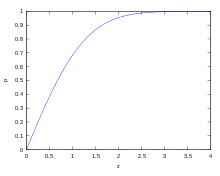
The probabilities for certain scattering intervals $[\mu -z\sigma ;\mu +z\sigma ]$ can be calculated as.

$p=2\Phi (z)-1$ ,

Where $\Phi (z)={\frac {1}{\sqrt {2\pi }}}\int _{-\infty }^{z}e^{-{\frac {x^{2}}{2}}}\,\mathrm {d} x$ is the distribution function of the standard normal distribution.

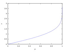
Conversely, for given can be given by $p\in (0,1)$

$z=\Phi ^{{-1}}\left({\frac {p+1}{2}}\right)$

the limits of the associated scattering interval $[\mu -z\sigma ;\mu +z\sigma ]$ with probability are calculated.

An example (with variation range)

Human height is approximately normally distributed. In a sample of 1,284 girls and 1,063 boys between the ages of 14 and 18, the average height of girls was measured to be 166.3 cm (standard deviation 6.39 cm) and the average height of boys was measured to be 176.8 cm (standard deviation 7.46 cm).

Accordingly, above range of variation suggests that 68.3% of girls have height in the range 166.3 cm ± 6.39 cm and 95.4% in the range 166.3 cm ± 12.8 cm,

16% [≈ (100% - 68.3%)/2] of girls are shorter than 160 cm (and 16% correspondingly taller than 173 cm); and
2.5% [≈ (100% - 95.4%)/2] of girls shorter than 154 cm (and 2.5% correspondingly taller than 179 cm).

For boys, 68% can be expected to have a height in the range 176.8 cm ± 7.46 cm and 95% in the range 176.8 cm ± 14.92 cm,

16% of boys smaller than 169 cm (and 16% larger than 184 cm) and
2.5% of boys are shorter than 162 cm (and 2.5% taller than 192 cm).

Coefficient of variation

From the expected value μ $\mu$ and standard deviation σ $\sigma$ of the ${\mathcal {N}}(\mu ,\sigma ^{2})$ distribution, we directly obtain the coefficient of variation

$\operatorname {VarK} ={\frac {\sigma }{\mu }}.$

Skew

The skewness $\sigma$ always has the value regardless of the parameters μ $\mu$ and σ $0$ .

Camber

The kurtosis is also $\sigma$ independent of μ $\mu$ and σ and is equal to . To better estimate the kurtosis of other distributions, they are often compared to the kurtosis of the normal distribution. In this case, the kurtosis of the normal distribution is $0$ normalized to (subtraction from 3); this quantity is called the excess.

Cumulants

The cumulant generating function is

$g_{X}(t)=\mu t+{\frac {\sigma ^{2}t^{2}}{2}}$

Thus the first cumulant is κ $\kappa _{1}=\mu$ , the second is κ $\kappa _{2}=\sigma ^{2}$ and all further cumulants vanish.

Characteristic function

The characteristic function for a standard normally distributed random variable $Z\sim {\mathcal {N}}(0,1)$ is

$\varphi _{Z}(t)=e^{-{\frac {1}{2}}t^{2}}$ .

For a random variable $X\sim {\mathcal {N}}(\mu ,\sigma ^{2})$ this gives $X=\sigma Z+\mu$ :

$\varphi _{X}(t)=\operatorname {E} (e^{it(\sigma Z+\mu )})=\operatorname {E} (e^{it\sigma Z}e^{it\mu })=e^{it\mu }\operatorname {E} (e^{it\sigma Z})=e^{it\mu }\varphi _{Z}(\sigma t)=\exp \left(it\mu -{\tfrac {1}{2}}\sigma ^{2}t^{2}\right)$ .

Moment generating function

The moment generating function of the normal distribution is

$m_{X}(t)=\exp \left(\mu t+{\frac {\sigma ^{2}t^{2}}{2}}\right)$ .

Moments

Let the random variable be ${\mathcal {N}}(\mu ,\sigma ^{2})$ -distributed. Then their first moments are as follows:

Order	Moment	central moment
	$\operatorname {E} (X^{k})$	$\operatorname {E} ((X-\mu )^{k})$
0
1	$\mu$	$0$
2	$\mu ^{2}+\sigma ^{2}$	$\sigma ^{2}$
3	$\mu ^{3}+3\mu \sigma ^{2}$	$0$
4	$\mu ^{4}+6\mu ^{2}\sigma ^{2}+3\sigma ^{4}$	$3\sigma ^{4}$
5	$\mu ^{5}+10\mu ^{3}\sigma ^{2}+15\mu \sigma ^{4}$	$0$
6	$\mu ^{6}+15\mu ^{4}\sigma ^{2}+45\mu ^{2}\sigma ^{4}+15\sigma ^{6}$	$15\sigma ^{6}$
7	$\mu ^{7}+21\mu ^{5}\sigma ^{2}+105\mu ^{3}\sigma ^{4}+105\mu \sigma ^{6}$	$0$
8	$\mu ^{8}+28\mu ^{6}\sigma ^{2}+210\mu ^{4}\sigma ^{4}+420\mu ^{2}\sigma ^{6}+105\sigma ^{8}$	$105\sigma ^{8}$

All central moments μ $\mu _{n}$ can be $\sigma$ represented by the standard deviation σ

$\mu _{n}={\begin{cases}0&{\text{wenn }}n{\text{ ungerade}}\\(n-1)!!\cdot \sigma ^{n}&{\text{wenn }}n{\text{ gerade}}\end{cases}}$

double faculty was used in the process:

$(n-1)!!=(n-1)\cdot (n-3)\cdot \ldots \cdot 3\cdot 1\quad \mathrm {f{\ddot {u}}r} \;n{\text{ gerade}}.$

Also for $X\sim {\mathcal {N}}(\mu ,\sigma ^{2})$ a formula for non-central moments can be given. For this one transforms $Z\sim {\mathcal {N}}(0,1)$ and applies the binomial theorem.

$\operatorname {E} (X^{k})=\operatorname {E} ((\sigma Z+\mu )^{k})=\sum _{j=0}^{k}{k \choose j}\operatorname {E} (Z^{j})\sigma ^{j}\mu ^{k-j}=\sum _{i=0}^{\lfloor k/2\rfloor }{k \choose 2i}\operatorname {E} (Z^{2i})\sigma ^{2i}\mu ^{k-2i}=\sum _{i=0}^{\lfloor k/2\rfloor }{k \choose 2i}(2i-1)!!\sigma ^{2i}\mu ^{k-2i}.$

Invariance to convolution

The normal distribution is invariant to the convolution, i.e., the sum of independent normally distributed random variables is again normally distributed (see also under stable distributions or under infinitely divisible distributions). Thus, the normal distribution forms a convolution semigroup in its two parameters. An illustrative formulation of this fact is: The convolution of a Gaussian curve of half-width Γ $\Gamma _{a}$ with a Gaussian curve of half-width Γ $\Gamma _{b}$ results again in a Gaussian curve with half-width

$\Gamma _{c}={\sqrt {\Gamma _{a}^{2}+\Gamma _{b}^{2}}}$ .

So if are X,Y two independent random variables with

$X\sim {\mathcal {N}}(\mu _{X},\sigma _{X}^{2}),\ Y\sim {\mathcal {N}}(\mu _{Y},\sigma _{Y}^{2}),$

then their sum is also normally distributed:

$X+Y\sim {\mathcal {N}}(\mu _{X}+\mu _{Y},\sigma _{X}^{2}+\sigma _{Y}^{2})$ .

This can be shown, for example, by using characteristic functions, using that the characteristic function of the sum is the product of the characteristic functions of the summands (cf. convolution theorem of the Fourier transform).

Given more generally independent and normally distributed random variables $X_{i}\sim {\mathcal {N}}(\mu _{i},\sigma _{i}^{2})$ . Then each linear combination is again normally distributed

$\sum _{i=1}^{n}c_{i}X_{i}\sim {\mathcal {N}}\left(\sum _{i=1}^{n}c_{i}\mu _{i},\sum _{i=1}^{n}c_{i}^{2}\sigma _{i}^{2}\right)$

in particular, the sum of the random variables is again normally distributed

$\sum _{i=1}^{n}X_{i}\sim {\mathcal {N}}\left(\sum _{i=1}^{n}\mu _{i},\sum _{i=1}^{n}\sigma _{i}^{2}\right)$

and the arithmetic mean also

${\frac {1}{n}}\sum _{i=1}^{n}X_{i}\sim {\mathcal {N}}\left({\frac {1}{n}}\sum _{i=1}^{n}\mu _{i},{\frac {1}{n^{2}}}\sum _{i=1}^{n}\sigma _{i}^{2}\right).$

According to Cramér's theorem, even the reverse is true: If a normally distributed random variable is the sum of independent random variables, then the summands are also normally distributed.

The density function of the normal distribution is a fixed point of the Fourier transform, i.e., the Fourier transform of a Gaussian curve is again a Gaussian curve. The product of the standard deviations of these corresponding Gaussian curves is constant; the Heisenberg uncertainty principle applies.

Entropy

The normal distribution has entropy: $\log \left(\sigma {\sqrt {2\,\pi \,e}}\right)$ .

Since for given expected value and given variance it has the largest entropy among all distributions, it is often used as a priori probability in the maximum entropy method.

Intervals around μ $\mu$ for normal distribution

Dependence of the scattering interval limit on the included probability z(p)

Dependence of the probability (percent within) on the size of the scatter interval p(z)

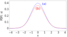
Normal distribution (a) and contaminated normal distribution (b)

Density of a centered normal distribution δ $\delta_{a}(x)=\tfrac {1}{\sqrt{\pi}a} \cdot e^{-\frac {x^2}{a^2}}$ .
For $a\to 0$ the function gets higher and narrower, but the area remains unchanged 1.

Relationships with other distribution functions

Transformation to standard normal distribution

A normal distribution with any μ $\mu$ and σ $\sigma$ and distribution function has the following relationship to the ${\mathcal {N}}(0,1)$ distribution, as mentioned above:

$F(x)=\Phi \left({\tfrac {x-\mu }{\sigma }}\right)$ .

In it is $\Phi$ the distribution function of the standard normal distribution.

If $X\sim {\mathcal {N}}(\mu ,\sigma ^{2})$ , then the standardization leads

$Z={\frac {X-\mu }{\sigma }}$

to a standard normally distributed random variable , because

$P(Z\leq z)=P\left({\tfrac {X-\mu }{\sigma }}\leq z\right)=P\left(X\leq \sigma z+\mu \right)=F(\sigma z+\mu )=\Phi (z)$ .

Geometrically, the substitution performed corresponds to an areal transformation of the bell curve of ${\mathcal {N}}(\mu ,\sigma ^{2})$ to the bell curve of ${\mathcal {N}}(0,1)$ .

Approximation of the binomial distribution by the normal distribution

→ Main article: Normal approximation

The normal distribution can be used to approximate the binomial distribution if the sample size is sufficiently large and the proportion of the sought property in the population is neither too large nor too small (Moivre-Laplace theorem, central limit theorem, for experimental confirmation see also under Galton board).

a Bernoulli experiment with independent stages (or random experiments) with a probability of success , the probability of successes can be $P(X=k)={\tbinom {n}{k}}\cdot p^{k}\cdot (1-p)^{n-k},\quad k=0,1,\dotsc ,n$ calculated in general by (binomial distribution).

This binomial distribution can be approximated by a normal distribution if sufficiently large and neither too large nor too small. As a rule of thumb, $np(1-p)\geq 9$ . For the expected value μ $\mu$ and the standard deviation σ $\sigma$ then holds:

$\mu =n\cdot p$ and σ $\sigma ={\sqrt {n\cdot p\cdot (1-p)}}$ .

Thus, for the standard deviation σ $\sigma \geq 3$ .

If this condition is not satisfied, the inaccuracy of the approximation is still acceptable if $np\geq 4$ and at the same time $n(1-p)\geq 4$ .

The following approximation is then useful:

${\begin{aligned}P(x_{1}\leq X\leq x_{2})&=\underbrace {\sum _{k=x_{1}}^{x_{2}}{n \choose k}\cdot p^{k}\cdot (1-p)^{n-k}} _{\mathrm {BV} }\\&\approx \underbrace {\Phi \left({\frac {x_{2}+0{,}5-\mu }{\sigma }}\right)-\Phi \left({\frac {x_{1}-0{,}5-\mu }{\sigma }}\right)} _{\mathrm {NV} }.\end{aligned}}$

In the normal distribution, the lower limit is reduced by 0.5 and the upper limit is increased by 0.5 to ensure a better approximation. This is also called "continuity correction". Only if σ $\sigma$ has a very high value, it can be dispensed with.

Since the binomial distribution is discrete, some points must be taken into account:

The difference between {\displaystyle $\leq$ (as well as between greater than and greater than or equal to) must be taken into account (which is not the case for the normal distribution). Therefore, for $P(X_{\text{BV}}<x)$ next smallest natural number must be chosen, i. e.

$P(X_{\text{BV}}<x)=P(X_{\text{BV}}\leq x-1)$ ( X $P(X_{\text{BV}}>x)=P(X_{\text{BV}}\geq x+1)$ ,

so that the normal distribution can be used for further calculations.

For example, $P(X_{\text{BV}}<70)=P(X_{\text{BV}}\leq 69)$

Besides

$P(X_{\text{BV}}\leq x)=P(0\leq X_{\text{BV}}\leq x)$

$P(X_{\text{BV}}\geq x)=P(x\leq X_{\text{BV}}\leq n)$

$P(X_{\text{BV}}=x)=P(x\leq X_{\text{BV}}\leq x)$ (necessarily with continuity correction)

and can thus be calculated by the formula given above.

The great advantage of the approximation is that very many levels of a binomial distribution can be determined very quickly and easily.

Relationship to Cauchy distribution

The quotient of two stochastically independent ${\mathcal {N}}(0,1)$ -standard normally distributed random variables is Cauchy distributed.

Relationship to Chi-Square Distribution

The square of a normally distributed random variable has a chi-squared distribution with one degree of freedom. Thus, if $Z\sim {\mathcal {N}}(0,1)$ , then $Z^{2}\sim \chi ^{2}(1)$ . Furthermore, if χ $\chi ^{2}(r_{1}),\chi ^{2}(r_{2}),\dotsc ,\chi ^{2}(r_{n})$ are jointly stochastically independent chi-squared distributed random variables, then

$Y=\chi ^{2}(r_{1})+\chi ^{2}(r_{2})+\dotsb +\chi ^{2}(r_{n})\sim \chi ^{2}(r_{1}+\dotsb +r_{n})$ .

From this follows with independent and standard normally distributed random variables $Z_{1},Z_{2},\dotsc ,Z_{n}$ :

$Y=Z_{1}^{2}+\dotsb +Z_{n}^{2}\sim \chi ^{2}(n)$

Other relationships are:

The sum $X_{n-1}={\frac {1}{\sigma ^{2}}}\sum _{i=1}^{n}(Z_{i}-{\overline {Z}})^{2}$ with ${\overline {Z}}:={\frac {1}{n}}\sum _{i=1}^{n}Z_{i}$ and independent normally distributed random variables $Z_{i}\sim {\mathcal {N}}(\mu ,\sigma ^{2}),\;i=1,\dotsc ,n$ satisfies a chi-squared distribution $X_{n-1}\sim \chi _{n-1}^{2}$ with degrees of freedom.

As the number of degrees of freedom increases (df ≫ 100), the chi-square distribution approaches the normal distribution.

The chi-square distribution is used for confidence estimation for the variance of a normally distributed population.

Relationship to Rayleigh distribution

The amount $Z={\sqrt {X^{2}+Y^{2}}}$ two independent normally distributed random variables X,Y , each with mean μ $\mu _{X}=\mu _{Y}=0$ and equal variances σ $\sigma _{X}^{2}=\sigma _{Y}^{2}=\sigma ^{2}$ , is Rayleigh distributed with parameter σ

Relationship to log normal distribution

If the random variable is normally distributed with ${\mathcal {N}}(\mu ,\sigma ^{2})$ , then the random variable $Y=e^{X}$ is log-normally distributed, so $Y\sim {\mathcal {LN}}(\mu ,\sigma ^{2})$ .

The emergence of a logarithmic normal distribution is due to multiplicative, that of a normal distribution to additive interaction of many random variables.

Relationship to F-Distribution

If the stochastically independent and identically-normally distributed random variables $X_{1}^{(1)},X_{2}^{(1)},\dotsc ,X_{n}^{(1)}$ and $X_{1}^{(2)},X_{2}^{(2)},\dotsc ,X_{n}^{(2)}$ have the parameters

$\operatorname {E} (X_{i}^{(1)})=\mu _{1},{\sqrt {\operatorname {Var} (X_{i}^{(1)})}}=\sigma _{1}$

$\operatorname {E} (X_{i}^{(2)})=\mu _{2},{\sqrt {\operatorname {Var} (X_{i}^{(2)})}}=\sigma _{2}$

then the random variable is subject to

$Y_{n_{1}-1,n_{2}-1}:={\frac {\sigma _{2}(n_{2}-1)\sum \limits _{i=1}^{n_{1}}(X_{i}^{(1)}-{\overline {X}}^{(1)})^{2}}{\sigma _{1}(n_{1}-1)\sum \limits _{j=1}^{n_{2}}(X_{i}^{(2)}-{\overline {X}}^{(2)})^{2}}}$

of an F-distribution with $((n_{1}-1,n_{2}-1))$ degrees of freedom. Here are

${\overline {X}}^{(1)}={\frac {1}{n_{1}}}\sum _{i=1}^{n_{1}}X_{i}^{(1)},\quad {\overline {X}}^{(2)}={\frac {1}{n_{2}}}\sum _{i=1}^{n_{2}}X_{i}^{(2)}$ .

Relationship to student's t-distribution

If the independent random variables $X_1, X_2, \dotsc, X_n$ are identically normally distributed with parameters μ $\mu$ and σ $\sigma$ then the continuous random variable is subject to

$Y_{n-1}={\frac {{\overline {X}}-\mu }{S/{\sqrt {n}}}}$

with sample mean ${\overline {X}}={\frac {1}{n}}\sum _{i=1}^{n}X_{i}$ and sample variance $S^{2}={\frac {1}{n-1}}\sum _{i=1}^{n}(X_{i}-{\overline {X}})^{2}$ a student t distribution with (n-1) degrees of freedom.

For an increasing number of degrees of freedom, the student t-distribution approaches the normal distribution more and more closely. As a rule of thumb, from approx. df>30 student t-distribution can be approximated by the normal distribution if required.

The student t-distribution is used for confidence estimation for the expected value of a normally distributed random variable with unknown variance.

Calculating with the standard normal distribution

In tasks where the probability for μ $\mu$ - ${\sigma }^{2}$ -normally distributed random variables is to be determined by the standard normal distribution, it is not necessary to go through the transformation given above every time. Instead, simply use the transformation

$Z={\frac {X-\mu }{\sigma }}$

used to generate an ${\mathcal {N}}(0,1)$ -distributed random variable

The probability for the event that, for example, [x,y] lies in the interval is equal to a probability of the standard normal distribution by the following conversion:

Basic questions

In general, the distribution function gives the area under the bell curve up to the value , i.e., it calculates the definite integral from $-\infty$ to

This corresponds to a searched probability in tasks, where the random variable is smaller or not larger than a certain number Because of the continuity of the normal distribution, it makes no difference whether r{\displaystyle $\leq$ is required, because e.g.

$P(X=3)=\int _{3}^{3}f(x)\mathrm {d} x=0$ and thus

Analogous applies to "larger" and "not smaller".

Because can only be smaller or larger than a boundary (or lie inside or outside two boundaries), two basic questions arise for tasks in probability calculations on normal distributions:

In a random experiment, what is the probability that the standard normally distributed random variable takes on at most the value ?

$P(Z\leq z)=\Phi (z)$

In school mathematics, the term left spike is occasionally used for this statement, since the area under the Gaussian curve runs from the left to the boundary. For negative values are also allowed. However, many tables of the standard normal distribution have only positive entries - because of the symmetry of the curve and the negativity rule

$\Phi (-z)\ =\ 1-\Phi (z)$

of the "left tip", however, this does not represent a restriction.

What is the probability that in a random experiment the standard normally distributed random variable takes at least the value ?

$P(Z\geq z)=1-\Phi (z)$

Here, the term right spike is occasionally used, with

$P(Z\geq -z)=1-\Phi (-z)=1-(1-\Phi (z))=\Phi (z)$

there is also a negativity rule here.

Since any random variable with the general normal distribution can be transformed into the random variable $Z={\frac {X-\mu }{\sigma }}$ with the standard normal distribution, the questions apply equally to both quantities.

Scattering range and antistray range

Often the probability for a scatter range is of interest, i.e. the probability that the standard normally distributed random variable takes values between $z_{1}$ and $z_{2}$

$P(z_{1}\leq Z\leq z_{2})=\Phi (z_{2})-\Phi (z_{1})$

In the special case of the symmetric scattering range ( $z_{1}=-z_{2}$ , with $z_{2}>0$ ) holds

${\begin{aligned}P(-z\leq Z\leq z)&=P(|Z|\leq z)\\&=\Phi (z)-\Phi (-z)\\&=\Phi (z)-(1-\Phi (z))\\&=2\Phi (z)-1.\end{aligned}}$

For the corresponding antistray range, the probability that the standard normally distributed random variable takes values outside the range between $z_{1}$ and $z_{2}$ increases:

$P(Z\leq z_{1}{\text{ oder }}Z\geq z_{2})=\Phi (z_{1})+(1-\Phi (z_{2})).$

Thus, for a symmetrical antistray region, the following follows

${\begin{aligned}P(Z\leq -z{\text{ oder }}Z\geq z)&=P(|Z|\geq z)\\&=\Phi (-z)+1-\Phi (z)\\&=1-\Phi (z)+1-\Phi (z)\\&=2-2\Phi (z).\end{aligned}}$

Scattering areas using the example of quality assurance

Both scatter ranges are of particular importance, for example, in the quality assurance of technical or economic production processes. Here there are tolerance limits to be observed $x_{1}$ and $x_{2}$ , where there is usually a largest still acceptable distance $\epsilon$ from the expected value μ $\mu$ (= the optimal target value) exists. The standard deviation σ $\sigma$ on the other hand, can be obtained empirically from the production process.

If specified $[x_{1};x_{2}]=[\mu -\epsilon ;\mu +\epsilon ]$ as the tolerance interval to be maintained, then (depending on the question) a symmetrical scattering or antistray range is present.

In the case of the scattering range applies:

The antistray area is then given by

$P(|X-\mu |\geq \epsilon )=1-\gamma$

or if no scatter range was calculated by

$P(|X-\mu |\geq \epsilon )=2\cdot \left(1-\Phi \left({\frac {\epsilon }{\sigma }}\right)\right)=\alpha .$

Thus, the result γ $\gamma$ is the probability of saleable products, while α $\alpha$ the probability of rejects, both depending on the specifications of μ $\mu$ , σ $\sigma$ and $\epsilon$ .

If it is known that the maximum deviation $\epsilon$ symmetric about the expected value, questions are also possible where the probability is given and one of the other quantities is to be calculated.

Testing for normal distribution

To check whether data are normally distributed, the following methods and tests can be used, among others:

Chi-square test
Kolmogorov-Smirnov test
Anderson-Darling test (modification of the Kolmogorov-Smirnov test)
Lilliefors test (modification of the Kolmogorov-Smirnov test)
Cramér-von Mises test
Shapiro-Wilk test
Jarque-Bera test
Q-Q plot (descriptive review)
Maximum likelihood method (descriptive test)

The tests have different properties in terms of the type of deviations from the normal distribution that they detect. For example, the Kolmogorov-Smirnov test is more likely to detect deviations in the center of the distribution than deviations at the edges, while the Jarque-Bera test is quite sensitive to strongly deviating individual values at the edges ("heavy edges").

In contrast to the Kolmogorov-Smirnov test, the Lilliefors test does not require standardization, i.e., μ $\mu$ and σ $\sigma$ the assumed normal distribution may be unknown.

With the help of quantile-quantile diagrams or normal-quantile diagrams, a simple graphical check for normal distribution is possible.
With the maximum likelihood method, the parameters μ $\mu$ and σ $\sigma$ the normal distribution can be estimated and the empirical data can be compared graphically with the fitted normal distribution.

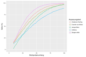
A χ²-distributed random variable with 5 degrees of freedom is tested for normal distribution. For each sample size, 10,000 samples are simulated and then 5 goodness-of-fit tests are performed at each 5% level.

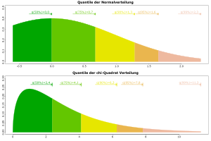
Quantiles of a normal distribution and a chi-square distribution

Parameter estimation, confidence intervals and tests

→ Main article: Normal distribution model

Many of the statistical problems in which the normal distribution occurs have been well studied. The most important case is the so-called normal distribution model, in which one assumes the performance of independent and normally distributed trials. Three cases occur in this process:

the expected value is unknown and the variance is known
the variance is unknown and the expected value is known
Expected value and variance are unknown.

Depending on which of these cases occurs, different estimators, confidence intervals or tests result. These are summarized in detail in the main article Normal Distribution Model.

The following estimators are of particular importance:

The sample means

${\overline {X}}={\frac {1}{n}}\sum _{i=1}^{n}X_{i}$

is an expectation-true estimator for the unknown expected value for both the case of a known and an unknown variance. It is even the best expectation-true estimator, i.e., the estimator with the smallest variance. Both the maximum likelihood method and the method of moments provide the sample mean as an estimator.

The uncorrected sample variance

$V(X)={\frac {1}{n}}\sum _{i=1}^{n}(X_{i}-\mu _{0})^{2}$ .

is an expectation-trusted estimator for the unknown variance given an expected value μ $\mu _{0}$ . It too can be obtained from both the maximum likelihood method and the method of moments.

The corrected sample variance

$V^{*}(X)={\frac {1}{n-1}}\sum _{i=1}^{n}(X_{i}-{\overline {X}})^{2}$ .

is an expectation-true estimator for the unknown variance with unknown expected value.

Applications outside the probability calculus

The normal distribution can also be used to describe facts that are not directly stochastic, for example in physics for the amplitude profile of Gaussian beams and other distribution profiles.

In addition, it is used in the Gabor transformation.

Questions and Answers

Q: What is the normal distribution?

A: The normal distribution is a probability distribution that is very important in many fields of science.

Q: Who discovered the normal distribution?

A: The normal distribution was first discovered by Carl Friedrich Gauss.

Q: What do location and scale parameters in normal distributions represent?

A: The mean ("average") of the distribution defines its location, and the standard deviation ("variability") defines the scale of normal distributions.

Q: How are the location and scale parameters of normal distributions represented?

A: The mean and standard deviation of normal distributions are represented by the symbols μ and σ, respectively.

Q: What is the standard normal distribution?

A: The standard normal distribution (also known as the Z distribution) is the normal distribution with a mean of zero and a standard deviation of one.

Q: Why is the standard normal distribution often called the bell curve?

A: The standard normal distribution is often called the bell curve because the graph of its probability density looks like a bell.

Q: Why do many values follow a normal distribution?

A: Many values follow a normal distribution because of the central limit theorem, which says that if an event is the sum of identical but random events, it will be normally distributed.