AlegsaOnline.com

Navier–Stokes equations: theory, applications, and mathematical challenges

Overview of the Navier–Stokes equations, their physical meaning, common forms, applications in science and engineering, and the central mathematical questions about existence and smoothness.

Author: Leandro Alegsa Creation date: November 13, 2022 Last updated: May 11, 2026

simple.wikipedia.org · CC BY-SA 4.0

Overview

The Navier–Stokes equations are the fundamental partial differential equations that govern the motion of viscous fluids. They express conservation of momentum (Newton's second law) together with mass conservation and relate velocity, pressure and external forces in a continuum description of liquids and gases. In modern presentations these equations are written as a system of partial differential equations for a velocity field and pressure, often supplemented by an incompressibility condition. The system arose historically from early work by Claude-Louis Navier and George Gabriel Stokes and has been refined to include various constitutive assumptions about stress and viscous diffusion.

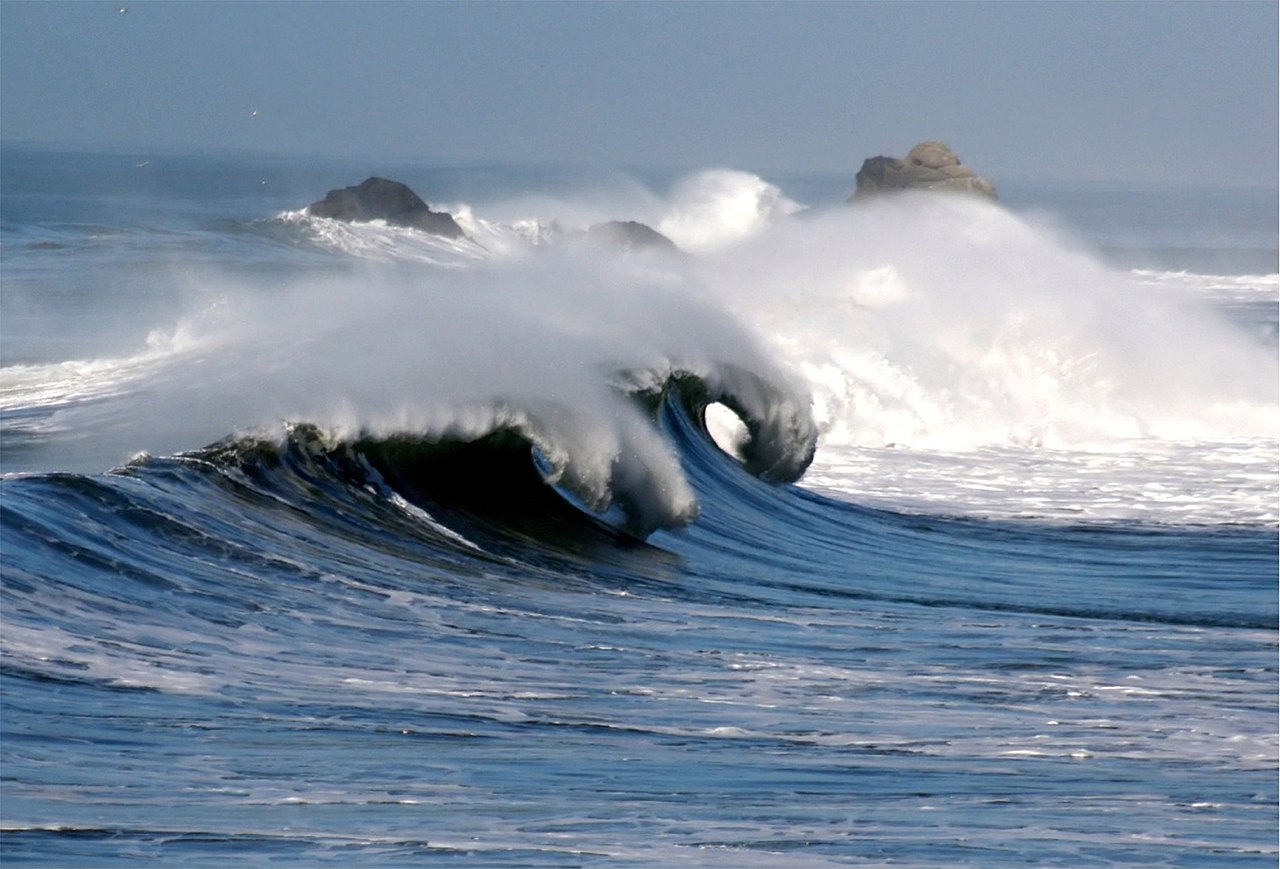
Form and physical interpretation

At its core the Navier–Stokes model balances inertial forces, pressure gradients and viscous stresses. One interprets the unknown as a velocity field that assigns a velocity vector to each point in space and time, rather than the trajectory of an individual particle. The viscous term represents momentum diffusion, often derived from a linear relation between stress and strain rate; the pressure term enforces local compression or expansion. External body forces such as gravity or electromagnetic forcing enter as source terms. In compact notation the equations link the time derivative and convective derivative of velocity to gradients of pressure and the Laplacian (or more general operators) representing viscous effects — an expression found in many textbooks and references on fluid mechanics.

Common simplified forms

Euler equations — the inviscid limit in which viscosity is neglected, appropriate for high‑Reynolds number flows where viscous forces are small (inviscid theory).
Stokes flow — the creeping‑flow limit where inertial terms are negligible compared with viscous terms, used for very slow or very small‑scale motions (low Reynolds).
Boundary layer equations — approximations that capture thin regions near solid surfaces where viscous effects concentrate (Prandtl).

Boundary conditions, solutions and visualization

To determine a unique solution one must prescribe boundary and initial conditions: for instance solid walls often impose a no‑slip velocity boundary condition, while inflow/outflow and symmetry conditions apply in other settings. Solutions are typically described by velocity and pressure fields; derived quantities such as vorticity, drag, lift, and volumetric flow rate are computed from those fields. For some problems analytical solutions exist in simple geometries, but most realistic configurations require numerical approximation by methods such as finite differences, finite volumes or spectral approaches (numerical methods). Visualization tools often render streamlines or particle traces to illustrate flow patterns (flow visualization).

Applications and examples

The Navier–Stokes equations underpin a wide range of applied science and engineering. They are central to weather and climate models that predict large‑scale atmospheric motion, to oceanography for currents and waves, to aerodynamics for air flow around wings and vehicles, and to hydrodynamics for pipe flow and river engineering. Biomedical uses include modelling blood flow in vessels; industrial applications cover combustion, process engineering and pollution dispersion. The equations also appear in multidisciplinary settings, for example in magnetohydrodynamics when coupled with electromagnetic equations to describe conducting fluids and plasmas (meteorology), (oceanography), (aerodynamics), (biomedical), (engineering).

Mathematical issues and open problems

Beyond practical modelling, the Navier–Stokes system presents deep mathematical challenges. In two spatial dimensions the theory of existence and regularity of solutions is well understood under broad conditions. In three spatial dimensions however, it remains unresolved whether smooth, globally defined solutions exist for all reasonable initial data or whether singularities (points where velocity becomes unbounded) can develop in finite time. This question, often called the Navier–Stokes existence and smoothness problem, is one of the famous Millennium Prize Problems highlighted by the Clay Mathematics Institute and discussed in many mathematical expositions (existence), (regularity), (singularity), (Millennium Prize), (open problems).

Computation, turbulence and practical considerations

In engineering practice, direct analytical solution is seldom possible, and numerical simulation (computational fluid dynamics) plays a central role. High‑resolution simulations can approximate laminar and turbulent flows, but turbulence presents additional complexity: energy cascades, sensitivity to small scales, and the need for modeling subgrid processes. Researchers employ techniques ranging from direct numerical simulation to Reynolds‑averaged models and large eddy simulation to manage computational cost while capturing essential physics (CFD), (turbulence modeling), (LES), (RANS). The development of stable, accurate solvers, appropriate boundary treatments and effective turbulence closures is an active area of research bridging mathematics, physics and engineering (numerical analysis), (software), (applications), (benchmarks).

Further reading typically covers continuum mechanics foundations, derivations from conservation laws, special exact solutions, asymptotic methods for thin or slow flows, and modern computational techniques; many introductory and advanced texts provide systematic treatments of the topics summarized here.

History

In 1686 Isaac Newton published his three-volume Principia containing the laws of motion and also defined the viscosity of a linearly viscous (today: Newtonian) fluid in the second book. In 1755 Leonhard Euler derived the Euler equations from the laws of motion, with which the behaviour of viscosity-free fluids (liquids and gases) can be calculated. The prerequisite for this was his definition of the pressure in a fluid, which is still valid today. Jean-Baptiste le Rond d'Alembert (1717-1783) introduced the Eulerian approach, derived the local mass balance and formulated the d'Alembert paradox, according to which no force is exerted on a body in the direction of flow by the flow of viscosity-free fluids (which Euler had already proved earlier). Because of this and other paradoxes of viscosity-free flows, it was clear that Euler's equations of motion had to be supplemented.

Claude Louis Marie Henri Navier, Siméon Denis Poisson, Barré de Saint-Venant and George Gabriel Stokes independently formulated the momentum theorem for Newtonian fluids in differential form in the first half of the 19th century. Navier (1827) and Poisson (1831) established the momentum equations after considering the action of intermolecular forces. In 1843 Barré de Saint-Venant published a derivation of the momentum equations from Newton's linear viscosity approach, two years before Stokes did so (1845). However, the name Navier-Stokes equations prevailed for the momentum equations.

Ludwig Prandtl made a significant advance in the theoretical and practical understanding of viscous fluids in 1904 with his boundary layer theory. From the middle of the 20th century, computational fluid dynamics developed to such an extent that with its help solutions of the Navier-Stokes equations can be found for practical problems, which - as has been shown - agree well with the real flow processes.

Simplifications

Due to the difficult solvability properties of the Navier-Stokes equations, one will try to consider simplified versions of the Navier-Stokes equations in the applications (as far as this is physically reasonable).

Euler equations

→ Main article: Euler's equations (fluid mechanics)

If the viscosity is neglected ( $\eta =\lambda =0$ ), one obtains the Euler equations (here for the compressible case)

$\rho {\frac {\partial {\vec {v}}}{\partial t}}+\rho ({\vec {v}}\cdot \nabla ){\vec {v}}=-\nabla p+{\vec {f}}.$

The Euler equations for compressible fluids play a role especially in aerodynamics as an approximation of the full Navier-Stokes equations.

Stokes equation

Another type of simplification is common, for example, in geodynamics, where the mantle of the Earth (or other terrestrial planets) is treated as an extremely viscous fluid (creeping flow). In this approximation, the diffusivity of momentum, i.e., the kinematic viscosity, is many orders of magnitude higher than the thermal diffusivity, and the inertia term can be neglected. Introducing this simplification into the stationary Navier-Stokes momentum equation, we obtain the Stokes equation:

$-\nabla p+\mu \cdot \Delta {\vec {v}}+{\vec {f}}=0$

Applying the Helmholtz projection to the equation, the pressure in the equation vanishes:

$\mu \cdot P\Delta {\vec {v}}+{\tilde {\vec {f}}}=0$

where ${\tilde {\vec {f}}}=P{\vec {f}}$ . This has the advantage that the equation now depends only on . ${\vec {v}}$ The original equation is obtained with

$\nabla p=(\operatorname {Id} -P)(\Delta {\vec {v}}+f),$

$P\Delta$ is also called the Stokes operator.

On the other hand, geomaterials have a complicated rheology, which leads to the fact that the viscosity is not considered constant. For the incompressible case this results:

$-\nabla p+\nabla \cdot \{\mu [\nabla {\vec {v}}+(\nabla {\vec {v}})^{\mathrm {T} }]\}+{\vec {f}}=0$

Boussinesq approximation

→ Main article: Boussinesq approximation

For gravity-dependent flows with small density variations and not too large temperature variations, the Boussinesq approximation is often used.