Logarithm — definition, properties, history and common uses

An accessible overview of logarithms: definition, basic properties and rules, common bases, historical development, practical uses and noteworthy distinctions.

Author: Leandro Alegsa Created: November 13, 2022 Updated: June 19, 2026

Overview

A logarithm, often shortened to "log", answers the question: "To what exponent must a given base be raised to produce a specified number?" In other words, if b^x = y, then x is the logarithm of y with base b and is written x = log_b(y). Logarithms are the inverse operation to exponentiation and are foundational in algebra, calculus and many applied fields. For further mathematical background see reference materials on logarithms.

Image gallery

8 Images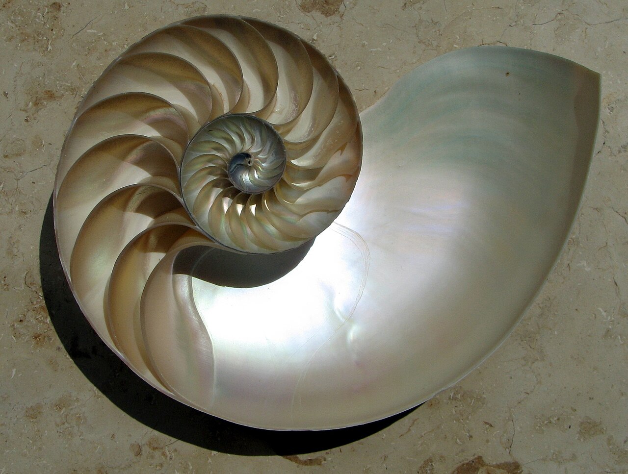

simple.wikipedia.org · CC BY-SA 3.0

Definition and parts

In the expression log_b(a) = c, the components are: the base b, the argument a (also called the input), and the result c (the exponent). The base is a positive real number not equal to 1, and the argument must be positive when working with real logarithms. The relation means b^c = a. Because logarithms undo exponentials, they convert multiplicative relationships into additive ones, which is the reason they are so useful in many calculations.

Basic properties and rules

Logarithms obey several algebraic rules that make them practical for manipulation and simplification of expressions. Common identities include:

Product rule: log_b(xy) = log_b(x) + log_b(y)
Quotient rule: log_b(x/y) = log_b(x) - log_b(y)
Power rule: log_b(x^k) = k · log_b(x)
Change of base: log_b(a) = log_c(a) / log_c(b), allowing conversion between different bases
Inverse relation: b^{log_b(a)} = a and log_b(b^x) = x (within domain restrictions)

Common bases and examples

Several bases are especially important in theory and applications. The binary logarithm (base 2), written log_2, is used in computer science to measure information and algorithmic complexity. The common logarithm (base 10), written log or log_{10}, was historically popular in engineering and was tabulated in tables used with slide rules. The natural logarithm, written ln or log_e, uses the base e (approximately 2.71828) and arises naturally in calculus, growth and decay models. For example, log_2(8) = 3 because 2^3 = 8. See examples of logarithmic calculations for worked examples.

$\log _{2}(8)=3\$

History and development

Logarithms were introduced in the early 17th century as a computational tool to simplify multiplication and division by transforming them into addition and subtraction. John Napier and others developed the idea, and Henry Briggs promoted base-10 tables that became widely used. The invention of logarithm tables and the later slide rule made large calculations much faster for scientists and engineers until electronic calculators and computers largely replaced those manual methods. For a historical overview consult history of logarithms.

$2^{3}=2\times 2\times 2=8\,$

Uses, examples and significance

Logarithms appear across mathematics and applied sciences. They are central in solving exponential equations, expressing scales that compress large ranges of values (for example, the Richter scale for earthquakes and decibel scale for sound), analyzing algorithmic complexity in computer science (e.g., O(log n) time), and modeling continuous growth or decay in natural sciences with the natural logarithm. In probability and statistics, log-likelihoods are commonly used because they turn products of probabilities into sums, simplifying optimization problems. For further reading on applications, see applied logarithms.

Notable distinctions and cautions

When working with real logarithms, remember the domain restrictions: the base must be positive and not equal to 1, and the argument must be positive. Complex logarithms extend the concept but require care because they are multi-valued. Also, while common and natural logs differ only by a constant scaling factor (a change of base), the context usually determines which base is most convenient: natural logs for calculus and continuous phenomena, base 2 for information theory, and base 10 for decadic scales and historical tabulations.

In summary, logarithms provide a powerful bridge between multiplication and addition, between exponential change and linear analysis, and between computations before calculators and modern numeric methods. They remain a basic and widely used tool across science, engineering and mathematics.

Logarithmic scale division of a slide rule (detail)

Graph of the logarithm function in base 2 (green), e (red) and 1/2 (blue)

In semi-logarithmic application (in relation to the x-axis), the graph of the logarithm function becomes a straight line. Shown here as an example for the logarithm to the base 10.

Overview

The use of the logarithm can be traced back to Indian antiquity. With the rise of banking and the progress of astronomy in 17th century Europe, the logarithm became increasingly important. Its function values were recorded in tables, the logarithmic tables, in order to be able to look them up and not always have to recalculate them. These tables were eventually replaced by slide rules and later by pocket calculators. The change from tables to slide rules took place in German schools in the 1960s, the change to pocket calculators from the 1970s.

Central aspects of life can be described with the help of logarithms. For example, the strength of a sensory impression increases as a function of a physical quantity such as brightness or volume according to the course of a logarithm function. The same applies to the perceived pitch as a function of the frequency of a tone.

Logarithms acquired their historical significance through the connection

$\log(xy) = \log x + \log y,$

which allows a multiplication to be expressed by an addition.

Formally, logarithms are all solutions of the equation

a = b^x

to given sizes and .

Depending on the range of numbers and the quantities for which this equation is considered, it has no solution, several solutions or exactly one solution. If the solution is unique, then it is called the logarithm of to the base and one writes

$x = \log_b a$

For example, the logarithm of 8 to the base 2 is equal to 3, written $\log_2 8 = 3$ because it is 2^3=8 .

If the above equation is to be solved for instead of , the solution is given by the th root of .

The best known and most widely used is the logarithm over the positive real numbers, which will be presented primarily in the following.

History

Indian mathematicians in the 2nd century BC were the first to mention logarithms. Even in ancient times, they used logarithms in base 2 for their calculations. In the 8th century, the Indian mathematician Virasena described logarithms in base 3 and 4. From the 13th century onwards, entire logarithmic tables were created by Arab mathematicians.

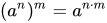Nicolas Chuquet clearly worked out the laws of arithmetic for powers $a^n\cdot a^m=a^{n+m}$ and $(a^n)^m = a^{n\cdot m}$ by a juxtaposition of an arithmetic and a geometric series.

The German mathematician Michael Stifel formulated similarly in 1544 the relations $q^m\cdot q^n = q^{m+n}$ and $\tfrac{q^m}{q^n} = q^{m-n}$ among other 16th century authors. The reduction of multiplication to addition, along with trigonometric addition formulae, stands at the beginning of the development of logarithms. Stifel allowed only whole-number exponents. John Napier's (1550-1617) idea, on the other hand, was to allow a continuous range of values for the exponents.

In the 17th century, the Swiss clockmaker Jost Bürgi (1552-1632) developed a new system for calculating logarithms, which he published in 1620 after much work. But even before that, in 1614, the Scottish thinker John Napier published a book on logarithms that made him famous as the "inventor of logarithms". However, Bürgi and Napier developed their work and findings on logarithms independently of each other.

The Greek word "logarithm" means "ratio" and comes from Napier. It is true that the same ratio to as to (as formula: a:b = c:d ) if the differences in their logarithms agree (as formula: $\log(a) - \log(b) = \log(c) - \log(d)$ ). Logarithms were first published by the latter under the title Mirifici logarithmorum canonis descriptio, which can be translated as Description of the Wonderful Canon of Logarithms.

After the Oxford professor Henry Briggs (1561-1630) had studied this writing intensively, he contacted its author and suggested using the base 10 for the logarithms (abbreviated lg). These spread quickly and were especially appreciated in astronomy, which Pierre-Simon Laplace also noted, in comparison to the trigonometric tables used before:

"L'invention des logarithmes, en réduisant le temps passé aux calculs de quelques mois à quelques jours, double pour ainsi dire la vie des astronomes."

"By reducing the time needed for calculations from a few months to a few days, the invention of logarithms has, so to speak, doubled the lifetime of an astronomer."

If the Euler number $\mathrm {e}$ - which was determined in 1728 by Leonhard Euler (1707-1783) and first published in 1742 - is used as the basis of the logarithm, it is called the natural logarithm. The natural logarithm is abbreviated by "ln".

With the logarithms, the mathematical basis for the further development of the mechanical slide rule was laid; for the functioning of the slide rule is based on the principle of addition and subtraction of logarithms.

Title page to Jost Bürgi's logarithm table from 1620

Logarithm in application and nature

Applications of the logarithm are often found in science when the range of values covers many orders of magnitude. Data are either represented with a logarithmic scale or logarithmically defined quantities are used, as for example with the pH value or the sensitivity of the sensory organs.

In the living nature

Numerous examples of logarithmic spirals can be found in living nature, such as the growth of snail shells or the arrangement of the seeds on the sunflower.

Sound pressure level

The sound pressure level is used as a logarithmic measure to describe the strength of a sound event. The auxiliary unit of measurement decibel (dB) is used for this purpose.

Brightness perception

A logarithmic evaluation has also proven itself for the sensory perception of brightness (Weber-Fechner law), since the human eye can bridge up to 10.5 powers of ten in physical luminance between twilight and bright sunshine.

pH value

The pH value is the measure of the acidic or basic character of an aqueous solution. Note: In chemistry, logarithmic scales are generally indicated by a preceding p (for power), for example in the pKS or pKB value.

Richter scale

The Richter scale, which is used to describe earthquake magnitudes, is based on a deca-logarithmic division. The earthquake magnitude therefore increases exponentially from level to level.

Star brightnesses

Star magnitudes are given in astronomical magnitude classes, which is a logarithmic measure of the actual radiant intensity.

Slide rule

Before electronic calculators were available, the laws of logarithms were exploited to simplify multiplications into additions and divisions into subtractions. The calculation of the square root is simplified at the level of the logarithm to a division by two. Because the logarithm itself is not so easy to calculate, slide rules with their logarithmic scale divisions and logarithm tables were widely used aids.

Growth and decay processes

Typical tasks in growth and decay processes can be modelled by the inverse function of the logarithm - the exponential function. See Exponential process, Absorption.

Number of digits of a number

Calculate the number of digits needed to represent a natural number in a place value system. To represent a natural number base , $1+\lfloor \log_b n \rfloor$ digits are needed. The brackets indicate rounding down to the nearest whole number that is less than or equal to.

For example, is $\log_2 100\approx 6{,}64$ . The above formula gives the value 7, so you need 7 digits to represent 100 in the dual system, namely 100=1100100_2 . If, on the other hand, you represent 100 in the hexadecimal system, you need two digits, because $\log_{16} 100\approx 1{,}66$ . It is $100=64_{16}$ .

Benford's Law

The distribution of the digits of numbers in empirical data sets, for example their first digits, follows a logarithmic distribution, Benford's law.

Information unit

Measurement of the amount of information; information theory says that if something occurs with probability knowing about the actual occurrence of it gives an amount of information of $\log_2 \tfrac 1p$ bit. For example, the result "heads" of a fair coin toss ( p=0{,}5 ) gives the amount of information $\log_2 2 = 1$ , and one bit is sufficient to encode this information.

Cryptography

The discrete logarithm is considerably more complicated to calculate in finite bodies and elliptic curves defined on them than its inverse function, the discrete exponential function. The latter can therefore be used as a so-called one-way function in cryptography for encryption.

Logarithmic time scales

Logarithmic time scales are found in the history of technology as well as in the geological time scale.

Intervals of music theory

Intervals have an exponential frequency progression. The auditory system, however, perceives them as linear. The proportions are therefore given as logarithms. The octave is divided into 1200 cents (music). Example:

Interval	Frequency ratio	Size
1 octave	2	1200 cents
2 octaves	4	2400 Cent
3 octaves	8	3600 Cent
…
major third	5:4	$1200\cdot \log _{2}{\big (}{\tfrac {5}{4}}{\big )}\,{\text{Cent}}=386{,}314\,{\text{Cent}}$
Fifth	3:2	$1200\cdot \log _{2}{\big (}{\tfrac {3}{2}}{\big )}\,{\text{Cent}}=701{,}955\,{\text{Cent}}$

Graphical representation of functions

Special mathematical papers are used for the graphical representation of functions, such as single-logarithmic paper or double-logarithmic paper.

The shell of a nautilus shows a logarithmic spiral

Designations

One writes for the logarithm of to the base

$x = \log_b a$

and says: " is the logarithm of to the base ". is called numerus or obsoletely also logarithmand. The result of logarithmising thus indicates with which exponent one must exponentiate the base } to obtain the numerus }.

For the digits before the decimal point of the logarithm, the term characteristic (sometimes also key figure) is usually used, its digits after the decimal point are called mantissa.

$\operatorname{log}_b a$

The general mathematical symbol for the logarithm according to DIN 1302. More rarely, one also finds notations deviating from it, such as ${}_b \,\!\log a$ .

$\operatorname{log}a$

The character $\log$ without a specified base is used when the base used is not important, is agreed separately, is obvious from the context or is specified by convention. In technical applications (such as on most pocket calculators), $\log$ often stands for the decadic logarithm. In theoretical papers, especially on number theory, $\log$ often stands for the natural logarithm.

In addition, special notations are specified for the logarithm in DIN 1302 depending on the application:

$\operatorname{ln}a$

Natural logarithm (Latin logarithmus naturalis), the logarithm to base $\mathrm {e}$ , the Eulerian number 2.7182818... It is used in connection with exponential functions.

$\operatorname{lg}a$

Decadic logarithm, also known as the logarithm of ten or Briggs logarithm, the logarithm to the base 10. It is used in numerical calculations in the decimal system.

$\operatorname{lb}a$

Binary logarithm, also called logarithm of two, the logarithm to the base 2. It is used in computer science for calculations in the binary system. Outside the standard, $\operatorname{ld}a$ - logarithmus dualis - is also used with the same meaning.

A similar looking function character is $\operatorname{li}a$ for the integral logarithm. However, this function is not a logarithm function.

Operating elements on a pocket calculator. The LOG key stands for the logarithm to base 10, LN calculates the natural logarithm to base e. In addition, the second assignment of the respective keys is the corresponding inverse function (yellow labelling above each), the exponential function to base 10 or e.

Definition

The logarithm can always be expressed mathematically as a set of functions (whose parameter is denoted by ) of $\R^+ \to \R$ can be understood. Their individual logarithm functions are only different (real but non-zero) multiples of each other.

Above the positive real numbers, it can be introduced in different ways. Depending on the background and intention, one or the other didactic approach will be chosen. The various definitions of the real logarithm are equivalent to each other and are given here with a special focus on the natural logarithm, which occurs naturally from the mathematician's point of view, as can be seen in the approach via the primitive function of $\tfrac{1}{t}$

As the inverse function of the exponential function

The logarithm to base is the inverse function of the general exponential function to positive base :

$x \mapsto b^x.$

The functions b^x and $\log_b x$ are therefore inverse functions of each other, i.e. logarithmising undoes exponentiation and vice versa:

$b^{\log_b x} = x \quad \text{und} \quad \log_b(b^x) = x.$

The natural logarithm is obtained with the base $b=\mathrm {e}$ , where

$\mathrm {e} =2{,}718281828459\ldots$

is the Euler number.

As a solution to a functional equation

The logarithm functions are the non-trivial, continuous solutions of the functional equation

$L(x \cdot y) = L(x) + L(y).$

Their solutions always satisfy L(1)=0 and even prove to be differentiable. The natural logarithm is then obtained together with the additional condition

L'(1) = 1.

The additional condition is one of the reasons for calling the logarithm obtained in this way natural. If one wanted to obtain the logarithm to a different base via the additional condition, then one would have to

$L'(1) = \frac 1{\ln b}$

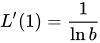
and would again require the natural logarithm.

The trivial solution of the above functional equation is the zero function L(x) = 0 which is not considered a logarithm function, and the only solution of the functional equation for which also L(0) defined.

Based on the above functional equation, the logarithm therefore conveys in particular a structure-preserving mapping from the positive real numbers with their multiplicative structure to the total real numbers with their additive structure. This can also be explicitly demanded as a condition and thus leads to the derivation.

As an isomorphism

The real-valued logarithms are exactly the continuous isomorphisms

$L\colon (\mathbb {R} ^{+}\!,\,\cdot \,)\longrightarrow (\mathbb {R} ,+)$ .

This definition uniquely defines the function except for one multiplicative constant.

The algebraic approach, like the approach via the functional equation, emphasises the historical significance of the logarithm as a calculation aid: it makes it possible to "convert" a multiplication into an addition.

As a primitive function of f with f(x)=1/x

The function

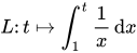
$L\colon t\mapsto \int _{1}^{t}{\frac {1}{x}}\,\mathrm {d} x$

with t>0 even the natural logarithm: it is L = ln The logarithm with base obtained by dividing the function by the constant $L(b)= \ln b$ . As an improper integral of , or any arbitrary (positive) lower limit of integration, one would only get one additional additive constant, but always only the logarithm to base $\mathrm {e}$ .

As a power series

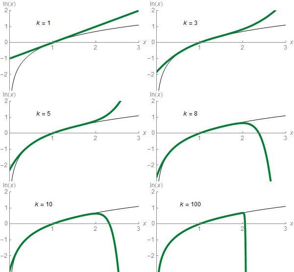
The natural logarithm can be expressed as a power series according to

$\ln(1+x) = \sum_{k=1}^\infty (-1)^{k+1} \frac{x^k}k = x-\frac{x^2}2 + \frac{x^3}3 -\frac{x^4}4 + \dotsb$

can be introduced. This series converges for |x|<1 for x = 1

For a numerical calculation of the value $\ln(1+x)$ for x>1 the relation $\ln(1+x)=-\ln {\Bigl (}1+{\Bigl (}-{\frac {x}{1+x}}{\Bigr )}{\Bigr )}$ useful.

Note

These definitions can also be used to obtain logarithms on other mathematical structures, such as the complex numbers. This assumes that the concepts used for the definition exist in the structure in question.

In order to define the discrete logarithm on a group, concepts such as differentiation/integration cannot be used because they do not exist there. (The definition happens there as an inversion of the exponentiation with whole exponents, which in turn is defined from multiple application of the one linkage of the group).

The natural logarithm as the area under the graph of 1/x

Calculation rules and basic properties

Logarithm laws

In the following it is always assumed that the variables x, y, x_i, r, a, b numbers are even assumed to be positive. Furthermore, the bases a,b of the logarithm must not be 1.

Products

For calculating with logarithms of products, there is the helpful calculation rule

$\log_b (x \cdot y) = \log_b x + \log_b y$

available; or more generally:

$\log _{b}(x_{1}x_{2}\dotsm x_{n})=\log _{b}x_{1}+\log _{b}x_{2}+\dotsb +\log _{b}x_{n}$

resp.

$\log_b\prod_{i=1}^n x_i = \sum_{i=1}^n \log_b x_i.$

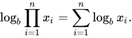
The logarithm of a product is the sum of the logarithms of the factors.

Ratios

The quotients are derived directly from the logarithms of products. Here only the simple case

$\log_b \frac xy = \log_b x - \log_b y$

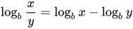
is given. The logarithm of a quotient is the logarithm of the numerator minus the logarithm of the denominator .

In particular, it follows (since $\log 1=0$ ):

$\log _{b}{\frac {1}{x}}=-\log _{b}x$

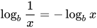
More generally, the reciprocity law results directly from the above quotient rule:

$\log _{b}{\frac {x}{y}}=-\log _{b}{\frac {y}{x}}$

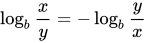
Totals and differences

From the formula for products, a formula for logarithms of sums (and differences) such as x+y derived by factoring out

$x+y=x\left(1+{\frac yx}\right).$

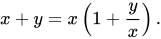
This results in the "rule

$\log _{b}(x+y)=\log _{b}x+\log _{b}\left(1+{\frac yx}\right).$

Powers

For powers with real exponent rule applies

$\log_b \left(x^r\right) = r \log_b x.$

The logarithm of a power is therefore the product of the exponent with the logarithm of the base.

Also from this, for r=-1

$\log_b \frac 1x = -\log_b x$

investigate.

The logarithm of a root fraction $\tfrac{1}{x}$ is the negative logarithm of the denominator .

These calculation rules can be derived from the power laws.

Roots

Since roots are nothing other than powers with fractional exponents, the power rule of the logarithm given above results in the calculation rule

$\log _{b}{\sqrt[{n}]{x}}=\log _{b}\left(x^{\frac {1}{n}}\right)={\frac {1}{n}}\log _{b}x.$

Base conversion

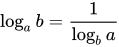
To calculate logarithms of base using logarithms of any base , use the relation

$\log_b x = \frac{\log_a x}{\log_a b}$

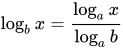
because with $y = \log_b x$ the transformations apply

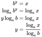
$\begin{align} b^y &= x \\ \log_a b^y &= \log_a x \\ y \log_a b &= \log_a x \\ y &= \frac{\log_a x}{\log_a b} \end{align}$

This shows that logarithms to different bases only differ from each other by a constant factor. Most spreadsheets provide logarithms only to base 10, pocket calculators also to base e (the natural logarithm). The above formula can be used to calculate logarithms to any base.

A prominent special case resulting from the above formula is:

$\log_a b = \frac{1}{\log_b a}$ or $\log_a b \cdot \log_b a=1$

Example

$\log_{10} 8 = \frac{\log_2 8}{\log_2 10} = \frac{\ln 8}{\ln 10}$

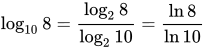
for any positive numbers is 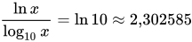$\frac{\ln x}{\log_{10} x} = \ln 10 \approx 2{,}302585$

Non-positive numbers

In the real numbers, the logarithm is not defined for non-positive numbers, i.e. zero and negative numbers. However, satisfies the $\log_b |x|$ above functional equation for $L(\cdot)$ , as long as only $x,y \not= 0$ since this has a discontinuity point there. Otherwise, for x=0 would always 0 = L(y) follow for all if one were to apply its validity to the whole of $\mathbb {R}$ , i.e. also at x=0 would be required.

$x=\log_b 0$ would then have to mean However, if is not zero, this is not solvable for any real
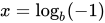
(as an example the negative number -1) would then have to $x=\log_b(-1)$ mean This is also not possible for any real number is greater than zero.

In function theory, where functions of complex numbers are considered, the logarithm can also be defined for negative numbers (see complex logarithm), but then some of the calculation rules no longer apply. In this context, 0 is also not an isolated singularity, but a branching point.

Derivative and integral

The natural logarithm function is the inverse function of the exponential function. Therefore, the derivative of the natural logarithm is obtained simply by applying the inverse rule (see example there). The result is

${\frac {{\mathrm d}}{{\mathrm d}x}}\ln(x)={\frac 1x}$

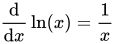
for positive . For negative it follows (because of $-x>0$ using the chain rule)

${\frac {{\mathrm d}}{{\mathrm d}x}}\ln(-x)={\frac {1}{-x}}\cdot (-1)={\frac 1x}$

and because 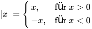$|x|=\begin{cases} x, & \text{für }x>0\\-x, & \text{für }x<0\end{cases}$ converted to

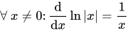
$\forall \ x\neq 0\colon {\frac {{\mathrm d}}{{\mathrm d}x}}\ln |x|={\frac 1x}$

summarise. The following applies to general logarithms:

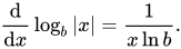
${\frac {{\mathrm d}}{{\mathrm d}x}}\log _{b}|x|={\frac 1{x\ln b}}.$

For all real $x\neq 0$ is

$\int_{-1}^x{\frac{1}{t}\,\mathrm dt} = \ln |x|,$

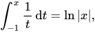
where for positive (i.e. when t=0 integrating over the pole at ) the principal value of the integral is to be taken.

The root function (also known as the indefinite integral) of the natural logarithm can be obtained by partial integration:

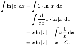
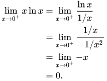
${\begin{aligned}\int {\ln |x|\,\mathrm {d} x}&=\int 1\cdot \ln |x|\,\mathrm {d} x\\&=\int {\frac {\mathrm {d} }{\mathrm {d} x}}x\cdot \ln |x|\,\mathrm {d} x\\&=x\ln |x|-\int x{\frac {1}{x}}\,\mathrm {d} x\\&=x\ln |x|\;-x+C.\end{aligned}}$

If, for a given integral of the natural logarithm, one of the limits is zero, de l'Hospital's rule can be applied.

Example

$\int_0^1{\ln x\,\mathrm dx} = [x\ln{x}-x]_0^1 = -1,$

$\begin{align} \lim_{x\to 0^+} x\ln x &= \lim_{x\to 0^+} \frac{\ln x}{1/x}\\ &= \lim_{x\to 0^+} \frac{1/x}{-1/x^2}\\ &= \lim_{x\to 0^+} -x\\ &= 0. \end{align}$

Curve discussion

Definition set: $\mathbb {R} ^{+}={\mathopen {]}}0,\infty {\mathclose {[}}$
Value set: $\mathbb {R}$
Zero point set or curve intersection points with the coordinate axes: {1} and (1|0) respectively.
Asymptotic behaviour:

$\lim _{x\to 0^{+}}\log _{b}x={\begin{cases}-\infty ,&{\text{wenn }}b>1\\+\infty ,&{\text{wenn }}b<1\end{cases}}$

$\lim _{x\to \infty }\log _{b}x={\begin{cases}+\infty ,&{\text{wenn }}b>1\\-\infty ,&{\text{wenn }}b<1\end{cases}}$

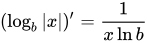
First derivative:

$(\log_b |x|)' = \frac 1{x\ln b}$

Extreme points: none
Turning points: none
Monotonicity: strictly monotonically (if decreasing (if b < 1
Area of the surface between curve, y-axis and x-axis up to x ≤ 1: $\frac {1}{|\ln b|}$
Curvature extremum at 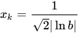$x_k=\frac{1}{\sqrt 2 |\ln b|}$ with κ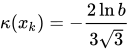 $\kappa(x_k) = -\frac{2\ln b}{3\sqrt 3}$

Natural logarithm

The logarithm to base $\mathrm {e}$ (of Euler's number) is also called the natural logarithm and is abbreviated as "ln" or often "log" (without subscript):

If $y=\mathrm {e} ^{x}$ , then $x=\log _{\mathrm {e} }y=\ln y$

or more simply formulated: $\ln(\mathrm {e} ^{x})=x$

The number $\mathrm {e}$ is distinguished (and could also be defined), for example, by the fact that the exponential function $\mathrm {e} ^{x}$ when derived with respect to , reproduces itself again, as a formula:

${\frac {\mathrm {d} }{\mathrm {d} x}}\mathrm {e} ^{x}=\mathrm {e} ^{x}.$

The term natural logarithm was chosen because both the exponential function and the logarithm to base $\mathrm {e}$ occur naturally without prefactors in many contexts (integral calculus, differential calculus, complex numbers, trigonometry). In particular, the natural logarithm can be integrated and differentiated very easily.

The natural logarithm $\ln$ is a root function of the reciprocal function with 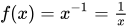$f(x)=x^{-1}=\tfrac{1}{x}$ namely exactly the one with F(1)=0 .

Calculation of the logarithm

The calculation of a logarithm is complicated in principle. It can only be achieved "with paper and pencil" by repeating certain calculation processes many times, whereby the result of the step just performed is used as the starting point for the next calculation step (iterative procedure). In most cases, the value can only be approximated (approximation). There are various possible procedures for this, some of which are shown below. Initially, the result of these partial steps is relatively far away from the correct result, but becomes more exact with each further calculation step, converging to the correct result. Such iterative arithmetic operations are very well suited to be performed automatically with a pocket calculator or computer, where only one key has to be pressed (if provided on the device) to calculate the logarithm of the entered number to a fixed base (usually Euler's number e (2.718...) or the number 10). The following calculation examples are each only suitable for calculating the logarithm of any number to the base e (natural logarithm) or 2.

Power series

The power series development of the natural logarithm around the development point 1 results for

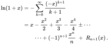
${\begin{aligned}\ln(1+x)&=-\sum _{k=0}^{\infty }{\frac {(-x)^{k+1}}{k+1}}\\&=x-{\frac {x^{2}}{2}}+{\frac {x^{3}}{3}}-{\frac {x^{4}}{4}}\pm \dotsb \\&\qquad \dotsb +(-1)^{n+1}{\frac {x^{n}}{n}}\;+\;R_{n+1}(x)\,.\end{aligned}}$

It does not converge very fast at the edges of the convergence interval, the remainder of the -th partial sum has the size

$|R_{n+1}(x)|\le\frac{|x|^{n+1}}{(n+1)(1-|x|)}.$

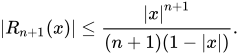
This series can also be represented as a continued fraction:

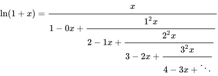
$\ln(1+x)={\cfrac {x}{1-0x+{\cfrac {1^{2}x}{2-1x+{\cfrac {2^{2}x}{3-2x+{\cfrac {3^{2}x}{4-3x+\ddots }}}}}}}}$

Using the formula $\ln(x)=m\ln(2)+\ln(2^{-m}x)$ one can reduce the calculation of the logarithm for any to that for values in the interval i.e., the calculation of the logarithm for any x {\displaystyle x} can be reduced to ${\big [}{\tfrac {2}{3}},{\tfrac {4}{3}}{\big ]}$ that for values in the interval [ 2 3 ]. h., one always finds and with 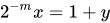$2^{-m}x=1+y$ and $|y|\le\tfrac13$

More flexibility in the reduction to numbers close to 1 and a halving of the computational effort is offered by the following series representation, which is based $\operatorname {artanh}$ on the power series expansion of the atranger hyperbolicus

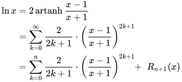
${\begin{aligned}\ln x&=2\operatorname {artanh} {\frac {x-1}{x+1}}\\&=\sum _{k=0}^{\infty }{\frac {2}{2k+1}}\cdot \left({\frac {x-1}{x+1}}\right)^{2k+1}\\&=\sum _{k=0}^{n}{\frac {2}{2k+1}}\cdot \left({\frac {x-1}{x+1}}\right)^{2k+1}\!\!+\,\,R_{n+1}(x)\end{aligned}}$

with the residual element estimation

$|R_{n+1}(x)|\leq {\frac {(x-1)^{2}}{2(2n+3)\,|x|}}\left|{\frac {x-1}{x+1}}\right|^{2n+1}.$

The series converges for x>0 , shows $\tfrac{1}{x}$ similar convergence behaviour for and converges better the closer } is to 1. To achieve this, one again uses

$\ln x = 2m \ln(\sqrt 2) + \ln(2^{-m} x).$

By choosing a suitable integer one can always achieve that 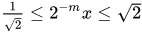$\tfrac1{\sqrt2} \leq 2^{-m}x \leq \sqrt2$ holds and thus increases the convergence speed of the series, which one now $2^{-m}x$ calculates for However, one must additionally 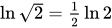$\ln\sqrt 2=\tfrac12\ln 2$ calculate an approximation for , which is done over the same series. Such a transformation to an interval ${\big [}{\tfrac {1}{b}},b{\big ]}$ by scaling with $b^{2m}$ is also possible for other values of , due to the particularly simple handling of the 2 numbers represented in binary, another factor is rarely used.

Additive decomposition

The natural logarithm $\ln$ per $\operatorname {artanh}$

$\ln x=2\operatorname {artanh} {\frac {x-1}{x+1}}\qquad \,(0<x)$

in relation to what is dissolved on the other side.

$\operatorname {artanh} u={\frac {1}{2}}\ln {\frac {1+u}{1-u}}\qquad (-1<u<1)$

results.

The logarithms of the positive integer numerals can thus be expressed in ascending ones of the form

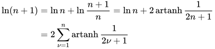
${\begin{aligned}\ln(n+1)&=\ln n+\ln {\frac {n+1}{n}}=\ln n+2\operatorname {artanh} {\frac {1}{2n+1}}\\&=2\sum _{\nu =1}^{n}\operatorname {artanh} {\frac {1}{2\nu +1}}\end{aligned}}$

and calculate it. This improves the convergence behaviour of the Taylor series

$\operatorname {artanh} u=\sum _{k=0}^{\infty }{\frac {u^{2k+1}}{2k+1}}=u+{\frac {1}{3}}u^{3}+{\frac {1}{5}}u^{5}+{\frac {1}{7}}u^{7}+\ldots$

slightly with increasing $n.$

With the help of the addition theorem

$\operatorname {artanh} u+\operatorname {artanh} v=\operatorname {artanh} {\frac {u+v}{1+uv}}$

$\operatorname {artanh}$ and thus also can be decomposed additively $\ln$ . Here, for the sake of clarity, the addition theorem is expressed as a group law $\oplus$

$u\oplus v:=\tanh(\operatorname {artanh} u+\operatorname {artanh} v)={\frac {u+v}{1+uv}},$

as well as its -fold multiplication as

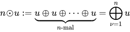
$n\!\odot \!u:=\underbrace {u\oplus u\oplus \dotsb \oplus u} _{n{\text{-mal}}}=\bigoplus _{\nu =1}^{n}u$

formulated.

$\tanh \left({\tfrac {1}{2}}\ln 2\right)$	$={\tfrac {1}{3}}$	$=2\!\odot \!{\tfrac {1}{7}}\;\oplus \;{\tfrac {1}{17}}$	$=\;\,7\!\odot \!{\tfrac {1}{19}}\;\ominus \;\;\,2\!\odot \!{\tfrac {1}{49}}\;\oplus \;3\!\odot \!{\tfrac {1}{161}},$
$\tanh \left({\tfrac {1}{2}}\ln 3\right)$	$={\tfrac {1}{2}}$	$=3\!\odot \!{\tfrac {1}{7}}\;\oplus \;2\!\odot \!{\tfrac {1}{17}}$	$=11\!\odot \!{\tfrac {1}{31}}\;\oplus \;\;\,8\!\odot \!{\tfrac {1}{49}}\;\oplus \;5\!\odot \!{\tfrac {1}{161}},$
$\tanh \left({\tfrac {1}{2}}\ln 5\right)$	$={\tfrac {2}{3}}$	$=4\!\odot \!{\tfrac {1}{5}}\;\ominus \;{\tfrac {1}{161}}$	$=16\!\odot \!{\tfrac {1}{31}}\;\oplus \;12\!\odot \!{\tfrac {1}{49}}\;\oplus \;7\!\odot \!{\tfrac {1}{161}},$
$\tanh \left({\tfrac {1}{2}}\ln 7\right)$	$={\tfrac {3}{4}}$	$=3\!\odot \!{\tfrac {1}{3}}\;\ominus \;{\tfrac {1}{15}}$	as well as $=14\!\odot \!{\tfrac {1}{15}}\;\oplus \;\;\,6\!\odot \!{\tfrac {1}{97}}\;\ominus \;3\!\odot \!{\tfrac {1}{127}}$
$\tanh \left({\tfrac {1}{2}}\ln 11\right)$	$={\tfrac {5}{6}}$	$=2\!\odot \!{\tfrac {1}{2}}\;\oplus \;{\tfrac {1}{10}}$	$=24\!\odot \!{\tfrac {1}{23}}\;\oplus \;11\!\odot \!{\tfrac {1}{65}}\;\ominus \;7\!\odot \!{\tfrac {1}{485}}.$

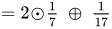
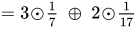
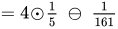
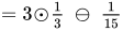
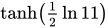
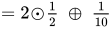
For practical calculations, decompositions are preferred whose summands have a one in the numerator. As in the case of the arc tangent, the doubling leaves

${\tfrac {1}{n}}=2\!\odot \!{\tfrac {1}{2n}}\;\oplus \;{\tfrac {1}{4n^{3}-3n}}$

get the ones in the counter.

Limit values according to Hurwitz

The following limits apply to the natural logarithm

$\ln x=\lim _{n\to \infty }n\left({\sqrt[{n}]{x}}-1\right)=\lim _{n\to \infty }n\left(1-{\frac {1}{\sqrt[{n}]{x}}}\right)$

and synonymously

$\ln x=\lim _{h\to 0}{\frac {x^{h}-1}{h}}=\lim _{h\to 0}\int _{1}^{x}{\frac {1}{t^{1-h}}}\,\mathrm {d} t$

which one can easily confirm with de l'Hospital's rule.

This is the basis for the limits of the sequences $a_{n}$ and given by Adolf Hurwitz for the natural logarithm. $b_{n}$ which are based on

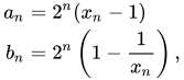
${\begin{aligned}a_{n}&=2^{n}(x_{n}-1)\\b_{n}&=2^{n}\left(1-{\frac {1}{x_{n}}}\right),\end{aligned}}$

where

$x_{n+1}=\sqrt{x_n}\quad\text{mit}\quad x_0=x$

are defined. Because $1-\tfrac1{x}\le b_n \le a_n < x-1$ because a n {\displaystyle $a_{n}$ decreasing and b n {\displaystyle $b_{n}$ increasing, the convergence of these two sequences follows. Due to a_n=b_n x_n and $x_{n}\rightarrow 1$ the equality of the two limit values results:

$\lim_{n\to\infty}a_n = \lim_{n\to\infty}b_n = \ln x.$

For a practical calculation of ln however, these limits are not well suited because of the cancellation that occurs.

Calculation of individual binary digits

Another way to calculate the logarithm is to determine the digits of the binary representation of the logarithm to the base 2 one after the other. This method is particularly easy to implement on arithmetic units, as it avoids time-consuming divisions and is also easy to convert to fixed-point arithmetic.

First, the digits before the decimal point of the two logarithm (always in the dual system) are determined by counting the digits before the decimal point of the number and normalised to values between 1 and 2 by shifting.

The logarithm of then has the representation

${\begin{aligned}\log _{2}(x)&=0,b_{1}b_{2}b_{3}\cdots =\sum _{k>0}b_{k}2^{-k}{\text{ mit }}b_{k}\in \{0,1\}\\\log _{2}(x^{2})&=b_{1},b_{2}b_{3}\cdots \qquad {\text{ wegen }}\quad \log(x^{2})=2\log x.\end{aligned}}$

Squaring thus shifts the logarithm one binary digit to the left, possibly making the pre-decimal place one. This is the case when $x^{2}\geq 2$ . In this case, normalised again by division by 2, which has no influence on the remaining decimal places. This results in the following sketch of the procedure:

INPUT 1 ≤ x < 2 OUTPUT Decimal places bi of _the binary representation of log2(x₎ i ← 0 LOOP i ← i + 1 x ← x2 IF x ≥ 2 THEN x ← x / 2 _bi ← 1 ELSE _bi ← 0 END IF END LOOP

Analogue computer

To calculate the logarithm with the aid of an analogue calculator - for example, the generation of an electrical output voltage $U_{\text{a}}$ which takes the logarithm of the nominal value of the input voltage $U_{\text{e}}$ can make use of the exponential course of the current-voltage characteristic of a diode. The sketch on the right shows the basic construction of a logarithmiser with an operational amplifier, a diode and a resistor .

Illustration of the first partial sums of the series representation of the natural logarithm discovered by Nicolaus Mercator; the series converges only in the non-hatched area

Illustration of the convergence of the adjacent artanh development for different numbers of summands

Simplified circuit diagram of a logarithmiser

Complex logarithm

Analogous to the real definition, each complex number is called which satisfies the equation

$\mathrm {e} ^{w}=z$

a natural logarithm of . For every $z\in \mathbb {C} \setminus \{0\}$ there exists such a which, however, in contrast to the real logarithm, because of

$\mathrm {e} ^{2k\pi \mathrm {i} }=1,\quad k\in \mathbb {Z}$ ,

is not uniquely determined. Thus, if one has found a logarithm of then also

$w'=\,\!w+2k\pi \mathrm {i}$

with each integer a logarithm of because it holds

$\mathrm {e} ^{w'}=\mathrm {e} ^{w+2k\pi \mathrm {i} }=\mathrm {e} ^{w}\cdot \mathrm {e} ^{2k\pi \mathrm {i} }=\mathrm {e} ^{w}\cdot 1=\mathrm {e} ^{w}=z$ .

To achieve uniqueness, one selects from the possible values for those values that lie in a suitable strip of the complex number plane. For example, one can use the strip

$\left\{w \in \mathbb C: -\pi < \operatorname{Im}\,w \leq \pi \right\}$

use. A value from this strip is called the principal value of the logarithm and is written 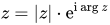$w = \ln z$ . If we set $z=|z|\cdot \mathrm {e} ^{\mathrm {i} \arg z}$ in polar form, one obtains a simple representation of the k-th branch of the logarithm function:

$w=\ln |z|+\mathrm {i} \left(\arg z+2k\pi \right),\quad k\in \mathbb {Z}$

with the argument function $\arg$ . In the summand $\ln |z|$ real logarithm already defined above is $\ln$ used. For k=0 the main branch of the complex logarithm is returned:

$\ln z=\ln |z|+\mathrm {i} \arg z$ .

$\ln$ is not continuous on $\mathbb C\setminus\{0\}$ . However, if one removes the negative real axis, $\ln$ on the domain is

$\mathbb C\setminus\{x \in \R: x\leq 0\}$

continuous and even holomorphic.

For attention

For the main branch of the complex logarithm $\ln$ not all of the above calculation rules for the real logarithm function apply. They apply only ${\text{mod }}2\pi \mathrm {i}$ . This ambiguity is a direct consequence of the periodicity of its inverse function, the complex exponential function. The comparison of

$\ln(-1+\mathrm {i} )+\ln(-1+\mathrm {i} )={\bigl (}\ln {\sqrt {2}}+{\frac {3\pi }{4}}\mathrm {i} {\bigr )}+{\bigl (}\ln {\sqrt {2}}+{\frac {3\pi }{4}}\mathrm {i} {\bigr )}=\ln 2+{\frac {3\pi }{2}}\mathrm {i}$

with

$\ln {\bigl (}(-1+\mathrm {i} )(-1+\mathrm {i} ){\bigr )}=\ln(-2\mathrm {i} )=\ln 2-{\frac {\pi }{2}}\mathrm {i}$

shows that

$\ln x + \ln y = \ln(x \cdot y)$

is not correct for all complex numbers and $0$ different from Also the equation

$y \cdot \ln x = \ln{x^y}$

is not always fulfilled, as the counterexample

$2\pi \mathrm {i} \ln \mathrm {e} =2\pi \mathrm {i} \;\neq \;0=\ln 1=\ln(\mathrm {e} ^{2\pi \mathrm {i} })$

proves.

· Graphical representation of the complex logarithm

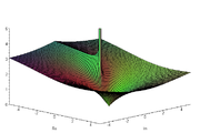
Amount of $\ln z$

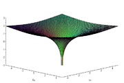
Real part of $\ln z$

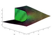
Imaginary part of $\ln z$

With the main branch of the complex logarithm defined above, one can explain the logarithm of negative real numbers:

$\ln(-x)=\ln \left\vert -x\right\vert +\mathrm {i} \arg(-x)=\ln x+\mathrm {i} \pi ,\quad x\in \mathbb {R} ^{+}\ .$

This requires that the argument function $\pi$ assigns the value π $\arg$ negative real numbers.

These considerations show that the ambiguity of the complex logarithm is ultimately due to the ambiguity of the argument function.

Riemann surface of the complex logarithm function: The leaves reflect the ambiguity of the logarithm, which follows from the periodicity of its inverse function, the exponential function.

Discrete logarithms

→ Main article: Discrete logarithm

Discrete logarithms are solutions of equations of the form

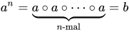
$a^{n}=\underbrace {a\circ a\circ \dotsb \circ a} _{n{\text{-mal}}}=b$

over a finite cyclic group $(G,\circ) = \langle a \rangle$ . The discrete logarithm of to the base is uniquely determined modulo the group order of and exists - since a producer of the group - for all elements of the group.

Discrete logarithms are complex to calculate for many groups in terms of complexity theory and are used in cryptography, for example in cryptosystems based on elliptic curves.

Example:

$2^{x}{\bmod {1}}1=5$

has the value 4 as a solution, because ²⁴ = 16 holds, and 16 leaves the remainder 5 when dividing with remainder by 11. The solution is unique modulo 10, i.e. modulo the group order of $(\mathbb Z\,/\,11 \,\mathbb Z)^\times$ . Accordingly, with also $x\pm 10$ is a solution of the congruence.

Questions and answers

Q: What are logarithms?

A: Logarithms are a part of mathematics related to exponential functions. They tell what exponent is needed to make a certain number, and they are the inverse of exponentiation.

Q: How were logarithms historically used?

A: Logarithms were historically useful in multiplying or dividing large numbers.

Q: What is an example of a logarithm?

A: An example of a logarithm is log₂(8)=3, where the base is 2, the argument is 8 and the answer is 3.

Q: What does this example mean?

A: This example means that two raised to the power of three (2³) equals eight (2x2x2=8).

Q: What are some common types of logarithms?

A: Some common types of logarithms include common logarithms with base 10, binary logarithms with base 2, and natural logarithms with base e ≈ 2.71828.

Author

AlegsaOnline.com Logarithm — definition, properties, history and common uses Leandro Alegsa

URL: https://en.alegsaonline.com/art/58853

How to cite this article

APA

Alegsa, L. (June 19, 2026). Logarithm — definition, properties, history and common uses. AlegsaOnline.com. https://en.alegsaonline.com/art/58853

MLA

Alegsa, Leandro. “Logarithm — definition, properties, history and common uses.” AlegsaOnline.com, June 19, 2026, https://en.alegsaonline.com/art/58853

Chicago

Alegsa, Leandro. “Logarithm — definition, properties, history and common uses.” AlegsaOnline.com. Updated June 19, 2026. https://en.alegsaonline.com/art/58853

BibTeX

@misc{alegsaonline_58853,
  author = {Alegsa, Leandro},
  title = {Logarithm — definition, properties, history and common uses},
  year = {2026},
  howpublished = {AlegsaOnline.com},
  url = {https://en.alegsaonline.com/art/58853},
  note = {Updated: June 19, 2026; Language: en}
}

TXT

Leandro Alegsa. “Logarithm — definition, properties, history and common uses.” AlegsaOnline.com. Updated: June 19, 2026. https://en.alegsaonline.com/art/58853

Sources

commons.wikimedia.org : Logarithm