Linear regression: concepts, history, methods, and practical uses
An accessible overview of linear regression covering its definition, mathematical form, history, assumptions, common estimation methods, extensions, and practical applications.
Overview
Linear regression is a family of statistical techniques used to describe and quantify a relationship between a measured outcome and one or more predictors. In its simplest form it fits a straight line that relates a dependent variable to an independent variable; more generally it models a dependent variable as a linear combination of several explanatory variables. The fitted relationship is used either to summarize how the outcome varies with predictors or to produce predictions for new observations.
Image gallery
1 Image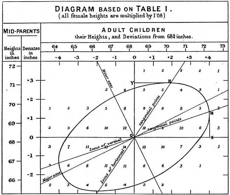
Basic form and key concepts
In algebraic terms a linear regression model expresses the dependent variable y as y = β0 + β1x1 + β2x2 + ... + βp xp + ε, where the β coefficients are parameters to be estimated and ε represents an error term. The model is called "linear" because it is linear in the unknown parameters β, even though predictors xj may be transformed (for example, squared or logged) before being entered into the model. Individual predictors are often referred to as explanatory variables.
Fitted values are obtained by choosing parameter estimates that make the discrepancies between observed outcomes and fitted values — called residuals — small according to some criterion. The most common criterion is the sum of squared residuals, known as ordinary least squares, but alternative criteria and penalties are frequently used depending on the goal and data characteristics.
Estimation, assumptions and diagnostic measures
Linear regression was one of the earliest systematic approaches to statistical modeling and occupies a central place in regression analysis. Estimation methods are simpler for models that are linear in their parameters because closed-form solutions or straightforward numerical procedures exist. When using standard ordinary least squares, analysts commonly invoke assumptions such as linearity in parameters, independence of errors, constant variance (homoscedasticity), and, for inferential statistics, approximate normality of residuals. Diagnostics include residual plots, tests for heteroscedasticity, and measures of fit such as R-squared.
History and development
The ideas behind least-squares fitting and linear approximation emerged in the late 18th and early 19th centuries. Early contributors developed methods to combine measurements and reduce error, and over time those ideas were formalized into estimation theory and the linear model framework used today. The mathematical convenience of linear-in-parameter models encouraged their early and widespread adoption in many scientific fields.
Common uses and examples
- Prediction and forecasting: build a model from historical data to predict future values of the dependent variable.
- Quantifying relationships: estimate the size and direction of association between outcome and individual predictors while holding others constant.
- Variable selection and explanation: identify which predictors are informative and which may be redundant or irrelevant.
- Baseline modeling: provide a simple interpretable benchmark before applying more complex methods.
Applications span economics, epidemiology, engineering, environmental science, and many other areas where a straightforward linear summary or predictive rule is useful.
Variations, extensions and alternatives
Although ordinary least squares is widely taught, practitioners often use variants tailored to particular challenges. The least-squares criterion itself is described in texts as least squares, and it can be modified or replaced. Robust alternatives minimize different norms or loss functions, for example methods that reduce sensitivity to outliers by minimizing absolute deviations rather than squared deviations; such approaches can be viewed as minimizing a lack-of-fit in another norm. When multicollinearity or overfitting is a concern, analysts add penalties to the least-squares objective — a class of techniques often called penalized methods — to shrink coefficient estimates toward zero.
More generally, the convenience of models that are linear in their unknown parameters has motivated wide use; however, for some problems statisticians employ nonlinear models or transform variables and still use least-squares style fitting procedures adapted to those settings.
Limitations and practical considerations
Linear regression produces interpretable coefficients but has limits. It assumes the specified linear form adequately captures relationships; it can perform poorly under strong nonlinearity or when predictors interact in complex ways. Extrapolation beyond the range of observed data is risky, and causal interpretation requires careful study design or additional assumptions. Good practice combines graphical checks, validation on held-out data, and consideration of alternative model forms when necessary.
Notable distinctions
Important distinctions include the difference between simple and multiple regression, and between models that are linear in parameters versus models that are linear in variables. Also, fitting by least squares is a method, while "linear model" describes a class of models — the two concepts often coincide but are not identical.
For readers seeking a practical introduction, many textbooks and online resources provide step-by-step examples, code snippets, and datasets that illustrate fitting, diagnosing, and interpreting linear regression models.
Further reading: introductory materials and more advanced treatments cover hypothesis testing for coefficients, confidence intervals, generalized least squares, and extensions to generalized linear models.
explanatory variables | regression analysis | unknown parameters | fitting | least squares | other norms | penalized methods
Questions and answers
Q: What is linear regression?
A: Linear regression is a way of looking at how something changes when other things change using math. It uses a dependent variable and one or more explanatory variables to create a straight line, known as the "line of regression".
Q: What are the advantages of linear regression?
A: The models which depend linearly on their unknown parameters are easier to fit than models which are non-linearly related to their parameters. Additionally, the statistical properties of the resulting estimators are easier to determine.
Q: What are some practical uses for linear regression?
A: Linear regression can be used to fit a predictive model to observed values (data) in order to make predictions, forecasts or reductions. It can also be used to quantify the strength of relationships between variables and identify subsets of data that contain redundant information about another variable.
Q: How do linear regression models try to minimize errors?
A: Linear regression models try to make the vertical distance between the line and the data points (the residuals) as small as possible. This is done by minimizing either the sum of squares of residuals (least squares), lack of fit in some other norm (least absolute deviations), or minimizing a penalized version of least squares loss function (ridge regression).
Q: Is it possible for linear regressions models not be based on least squares?
A: Yes, it is possible for linear regressions models not be based on least squares but instead use methods such as minimizing lack of fit in some other norm (least absolute deviations) or minimizing a penalized version of least squares loss function (ridge regression).
Q: Are “linear model” and “least squares” synonyms?
A: No, they are not synonyms. While they are closely linked, "linear model" refers specifically to using a straight line while "least squares" refers specifically to trying minimize errors by making sure that there is minimal vertical distance between the line and data points.
Related articles
Author
AlegsaOnline.com Linear regression: concepts, history, methods, and practical uses Leandro Alegsa
URL: https://en.alegsaonline.com/art/58267