Least squares

This article deals with the numerical aspects of this method. For a stochastic view, see Linear Simple Regression and Multiple Linear Regression.

The method of least squares (abbreviated MKQ or method of least squares, or simply least squares, abbreviated LS; to distinguish it from extensions derived from it, such as the generalized method of least squares, or the two-stage method of least squares, also referred to as "ordinary", i.e. ordinary least squares (OLS), or KQ method (obsolete method of least squares sum, abbreviated: LS) is the standard mathematical method for calculating the sum of the variance squares. (i.e. ordinary least squares (OLS) method), or KQ method (obsolete least squares method) is the standard mathematical procedure for the adjustment calculation. In this method, a function is determined for a set of data points that runs as close as possible to the data points and thus summarizes the data in the best possible way. The most commonly used function is the straight line, which is then called the equalization line. In order to use the method, the function must contain at least one parameter. These parameters are then determined by the method so that when the function is compared to the data points and the distance between the function value and the data point is squared, the sum of these squared distances becomes as small as possible. The distances are then called residuals.

Typically, this method examines real data, such as physical or economic measurements. These data often contain unavoidable measurement errors and fluctuations. With the assumption that the measured values are close to the underlying "true values" and that there is a certain relationship between the measured values, the method can be used to find a function that describes this relationship of the data as well as possible. The method can also be used in reverse to test different functions and thereby describe an unknown relationship in the data.

In the example graphic, data points and a compensation function are entered. A general function (the model function) is selected, which should fit the problem and the data, here a logistic function. Its parameters are now determined so that the sum of the deviation squares the observations from the values of the function is minimized. In the graph, the deviation at the point be seen as the perpendicular distance of the observation from the curve.

In stochastics, the least squares method is most often used as a regression analytical estimation method, where it is also referred to as least squares estimation or ordinary least squares estimation. Since least squares estimation minimizes the residual sum of squares, it is the estimation method that maximizes the coefficient of determination. Applied as system identification, the method of least squares in connection with model tests is e.g. for engineers a way out of the paradoxical situation to determine model parameters for unknown regularities.

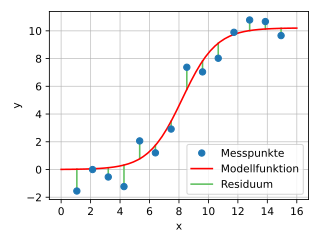
Measurement points and their distance from a function determined by the method of least squares. Here, a logistic function was chosen as the model curve.

History

On New Year's Day 1801, the Italian astronomer Giuseppe Piazzi discovered the dwarf planet Ceres. He was able to follow its orbit for 40 days, then Ceres disappeared behind the Sun. In the course of the year, many scientists unsuccessfully tried to calculate the orbit on the basis of Piazzi's observations - assuming a circular orbit, because only for such orbits could the orbital elements be mathematically determined from observed celestial positions at that time.

The 24-year-old Gauss managed to calculate the orbit with the help of a new indirect method of orbit determination and his balancing calculations based on the method of least squares (although not yet so called) in such a way that Franz Xaver von Zach was able to find it again on December 7, 1801, and - confirmed - on December 31, 1801. Heinrich Wilhelm Olbers confirmed this independently of Zach by observation on January 1 and 2, 1802.

The problem of the recovery of Ceres as such lay in the fact that by the observations neither the place, a piece of the orbit, nor the distance are known, but only the directions of the observation. This leads to the search of an ellipse and not of a circle, as Gauss' competitors assumed. One of the foci of the ellipse is known (the Sun itself), and the arcs of Ceres' orbit between the directions of observation are traversed according to Kepler's second law, that is, the times behave like the areas swept by the guiding ray. Moreover, for the computational solution, it is known that the observations themselves start from a conic section in space, the Earth's orbit itself.

In principle, the problem leads to an eighth-degree equation whose trivial solution is the Earth's orbit itself. Through extensive constraints and (later) the method of least squares developed by Gauss, the 24-year-old succeeded in giving the location he had calculated for Ceres' orbit for November 25 to December 31, 1801. This enabled Zach to find Ceres on the last day of the prediction. The location was no less than 7° (i.e. 13.5 full moon latitudes) east of where the other astronomers had suspected Ceres to be, which was duly appreciated not only by Zach but also by Olbers.

His first calculations were still without the method of the smallest squares, only when after the rediscovery of Ceres many new data were available, he used these for a more exact determination of the orbital elements, however, without disclosing details of his method generally. Piazzi's reputation, which had suffered greatly due to his orbital points not fitting a circular orbit, was also restored.

A predecessor method of the least squares method is the method of least absolute deviations, which was developed by Rugjer JosipBošković in 1760. Gauss had already developed the basics of the least squares method in 1795 at the age of 18. It was based on an idea of Pierre-Simon Laplace to sum up the deviations of the measured values from the expected value in such a way that the sum over all these so-called errors was zero. In contrast to this method, Gauss used the error squares instead of the errors and was thus able to dispense with the zero-sum requirement. Independently of Gauss, the Frenchman Adrien-Marie Legendre developed the same method, was the first to publish it in 1805, at the end of a small work on the calculation of comet orbits, and published a second treatise on it in 1810. His presentation was exceedingly clear and simple. Legendre also gave the name Méthode des moindres carrés (method of least squares).

In 1809, in the second volume of his celestial mechanics work Theoria motus corporum coelestium in sectionibus conicis solem ambientium (Theory of the motion of celestial bodies orbiting the sun in conic sections), Gauss published the method including the normal equations, as well as the Gaussian elimination method and the Gauss-Newton method, thus going far beyond Legendre. In it, he referred to the method of least squares as his discovery and claimed to have discovered and applied it already in 1795 (i.e. before Legendre), which annoyed the latter permanently. Legendre complained about this in a long letter to Gauss, which the latter left unanswered. Gauss only occasionally referred to an entry in his mathematical diary of June 17, 1798 (there is the cryptic sentence in Latin: Calculus probabilitatis contra La Place defensus (Calculus of probability defended against Laplace) and nothing else). Laplace judged the matter in such a way that Legendre made the first publication, but Gauss knew the method without doubt already before, used it himself and communicated it also to other astronomers by letter. After its publication, the method of least squares quickly became the standard procedure for the treatment of astronomical or geodetic data sets.

Gauss used the method intensively in his survey of the Kingdom of Hanover by triangulation. In 1821 and 1823 the two-part work and in 1826 a supplement to the Theoria combinationis observationum erroribus minimis obnoxiae (Theory of the combination of observations subjected to the smallest errors) were published, in which Gauss justified the success of the method of least squares by the fact that this is optimal in a broad respect in comparison with other methods of the adjustment calculation. The mathematical formulation of this statement is known as the Theorem of Gauss-Markov, named after Andrei Andreyevich Markov, who rediscovered and popularized this initially little-noticed part of Gauss's work in the 20th century (see also Theorem of Gauss-Markov#History). The Theoria Combinationis also contains methods for efficiently solving systems of linear equations, such as the Gauss-Seidel method and the LR decomposition, which represent a significant advance on the state of mathematical knowledge at the time.

The French survey officer André-Louis Cholesky developed the Cholesky decomposition during the First World War, which again represented a considerable gain in efficiency compared to the solution methods of Gauss. In the 1960s, Gene Golub developed the idea of solving the occurring linear systems of equations by means of QR decomposition.

Carl Friedrich Gauss

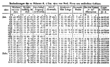
Piazzi's observations published in the Monatliche Correspondenz of September 1801

The procedure

Requirements

Consider a dependent variable which is influenced by one variable or by several variables. For example, the elongation of a spring depends only on the applied force, but the profitability of a company depends on several factors such as sales, the various costs or the equity. To simplify the notation, in the following the representation is limited to one variable The relationship between and the variables is described by a model function for example a parabola or an exponential function.

$y(x)=f(x;\alpha _{1},\dotsc ,\alpha _{m})$ ,

which depends on and on function parameters α $\alpha _{j}$ This function comes either from the user's knowledge or from a more or less complex search for a model, possibly different model functions have to be applied and the results compared. A simple case based on existing knowledge is for example the spring, because here Hooke's law and thus a linear function with the spring constant as the only parameter is a model prerequisite. In more difficult cases, however, such as that of the company, the choice of the function type must be preceded by a complex modeling process.

To obtain information about the parameters and thus the concrete nature of the relationship, for each given values $x_{i}$ the independent variables corresponding observed values $y_{i}$ $(i=1,\dotsc ,n)$ collected. The parameters α $\alpha _{j}$ are used to fit the chosen function type to these observed values $y_{i}$ . The goal is now to choose the parameters α $\alpha _{j}$ such that the model function approximates the data as best as possible.

Gauss and Legendre had the idea to make distributional assumptions about the measurement errors of these observed values. They should be zero on average, have a constant variance and be stochastically independent of any other measurement error. This requires that there is no systematic information in the measurement errors, i.e. that they fluctuate around zero purely by chance. In addition, the measurement errors should be normally distributed, which on the one hand has probabilistic advantages and on the other hand guarantees that outliers in good as excluded.

To determine the parameters α {\displaystyle $\alpha _{j}$ under these assumptions, it is generally necessary to have significantly more data points than parameters, so must n>m

Minimization of the sum of the squares of the errors

The criterion for determining the approximation should be chosen so that large deviations of the model function from the data are weighted more heavily than small ones. If no solution without deviations is possible, the compromise with the smallest overall deviation is the best generally valid criterion.

For this purpose, the sum of squared errors, also called the sum of squared errors (more precisely, the sum of squared residuals), is $y_{i}$ defined as the sum of squared differences between the values of the model curve $f(x_{i})$ and the data

In formula notation with parameters α ${\vec {\alpha }}=(\alpha _{1},\alpha _{2},\dots ,\alpha _{m})\in \mathbb {R} ^{m}$ and ${\vec {f}}=(f(x_{1},{\vec {\alpha }}),\dots ,f(x_{n},{\vec {\alpha }}))\in \mathbb {R} ^{n}$ results in

$\sum _{i=1}^{n}(f(x_{i},{\vec {\alpha }})-y_{i})^{2}=\|{\vec {f}}-{\vec {y}}\|_{2}^{2}.$

The parameters α for which the sum of squared fitting errors becomes minimal should then be $\alpha _{j}$ selected:

$\min _{\vec {\alpha }}\|{\vec {f}}-{\vec {y}}\|_{2}^{2}.$

Exactly how this minimization problem is solved depends on the nature of the model function.

When the error sum of squares is predicted for an external data set, it is referred to as the PRESS statistic (predictive residual sum of squares).

Linear model function

Linear model functions are linear combinations of arbitrary, generally non-linear basis functions. For such model functions, the minimization problem can also be solved analytically using an extremal approach without iterative approximation steps. First, some simple special cases and examples are shown.

Special case of a simple linear compensation line

Derivation and method

A simple model function with two linear parameters represents the first order polynomial

$f(x)=\alpha _{0}+\alpha _{1}x$

is displayed. For given measured values $(x_{1},y_{1}),\dotsc ,(x_{n},y_{n})$ the coefficients α $\alpha _{0}$ and α $\alpha _{1}$ the best-fitted straight line are searched. The deviations $r_{i}$ between the searched straight line and the respective measured values

${\begin{matrix}r_{1}=&\alpha _{0}+&\alpha _{1}x_{1}-y_{1}\\r_{2}=&\alpha _{0}+&\alpha _{1}x_{2}-y_{2}\\\vdots &\vdots &\vdots \\r_{n}=&\alpha _{0}+&\alpha _{1}x_{n}-y_{n}\\\end{matrix}}$

are called fitting errors or residuals. We are now looking for the coefficients α $\alpha _{0}$ and α $\alpha _{1}$ with the smallest sum of the error squares

$\min _{\alpha _{0},\alpha _{1}}\sum _{i=1}^{n}r_{i}^{2}$ .

The great advantage of the approach with this square of the errors becomes visible when this minimization is performed mathematically: The sum function is taken as a function of the two variables α $\alpha _{0}$ and α $\alpha _{1}$ (the incoming measured values are numerical constants in this case), then the derivative (more precisely: partial derivatives) of the function according to these variables (i.e. α $\alpha _{0}$ and α $\alpha _{1}$ ) and finally find the zero of this derivative. This results in the linear system of equations

${\begin{aligned}\textstyle n\cdot \alpha _{0}+\left(\sum \limits _{i=1}^{n}x_{i}\right)\alpha _{1}&=\textstyle \sum \limits _{i=1}^{n}y_{i}\\\textstyle \left(\sum \limits _{i=1}^{n}x_{i}\right)\alpha _{0}+\left(\sum \limits _{i=1}^{n}x_{i}^{2}\right)\alpha _{1}&=\textstyle \sum \limits _{i=1}^{n}x_{i}y_{i}\end{aligned}}$

with the solution

$\alpha _{1}={\frac {\sum \nolimits _{i=1}^{n}(x_{i}-{\overline {x}})y_{i}}{\sum \nolimits _{i=1}^{n}(x_{i}-{\overline {x}})^{2}}}={\frac {\sum \nolimits _{i=1}^{n}(x_{i}-{\overline {x}})(y_{i}-{\overline {y}})}{\sum \nolimits _{i=1}^{n}(x_{i}-{\overline {x}})^{2}}}={\frac {SP_{xy}}{SQ_{x}}}$ and α $\;\alpha _{0}={\overline {y}}-\alpha _{1}{\overline {x}}$ ,

where $SP_{xy}$ represents the sum of the deviation products between and , and $SQ_{x}$ represents the sum of the deviation squares of Here $\textstyle {\overline {x}}={\frac {1}{n}}\sum \nolimits _{i=1}^{n}x_{i}$ the arithmetic mean of the values, ${\overline {y}}$ correspondingly. The solution for α $\alpha _{1}$ can also be obtained in non-centered form using the displacement theorem

$\alpha _{1}={\frac {\sum _{i=1}^{n}(x_{i}y_{i})-n{\overline {x}}{\overline {y}}}{\left(\sum _{i=1}^{n}x_{i}^{2}\right)-n{\overline {x}}^{2}}}$

can be given. These results can also be derived with functions of a real variable, i.e. without partial derivatives.

Example with a compensation line

In this example, a compensation line of the form $f(x)=\alpha _{0}+\alpha _{1}x$ is calculated to represent the relationship between two features of a data set. The data set consists of length and width of ten warships (see warship data). An attempt will be made to relate the latitude to the longitude. The data is shown in the following table in the first three columns. The other columns refer to intermediate results for the calculation of the compensation lines. The variable $x_{i}$ shall denote the length of the warship and $y_{i}$ its width. The straight line $f(x)=y=\alpha _{0}+\alpha _{1}x$ is sought for which, if the known values $x_{i}$ substituted, the function values are as close as possible to the $f(x_{i})={\tilde {y}}_{i}$ known values $y_{i}$

Warship	Length (m)	Width (m)	$(x_{i}-{\overline {x}})$	$(y_{i}-{\overline {y}})$
	$x_{i}$	$y_{i}$	*$x_{i}^{}$**	*$y_{i}^{}$**	*$x_{i}^{}\cdot y_{i}^{}$*	*$(x_{i}^{})^{2}$**	$f(x_{i})$	$f(x_{i})-y_{i}$
1	208	21,6	40,2	3,19	128,24	1616,04	24,88	3,28
2	152	15,5	−15,8	−2,91	45,98	249,64	15,86	0,36
3	113	10,4	−54,8	−8,01	438,95	3003,04	9,57	−0,83
4	227	31,0	59,2	12,59	745,33	3504,64	27,95	−3,05
5	137	13,0	−30,8	−5,41	166,63	948,64	13,44	0,44
6	238	32,4	70,2	13,99	982,10	4928,04	29,72	−2,68
7	178	19,0	10,2	0,59	6,02	104,04	20,05	1,05
8	104	10,4	−63,8	−8,01	511,04	4070,44	8,12	−2,28
9	191	19,0	23,2	0,59	13,69	538,24	22,14	3,14
10	130	11,8	−37,8	−6,61	249,86	1428,84	12,31	0,51
Sum Σ	1678	184,1			3287,82	20391,60

The compensation line is determined by the coefficients α $\alpha _{0}$ and α $\alpha _{1}$ , which are calculated as above with

$\alpha _{1}={\frac {\sum \nolimits _{i=1}^{n}(x_{i}-{\overline {x}})(y_{i}-{\overline {y}})}{\sum \nolimits _{i=1}^{n}(x_{i}-{\overline {x}})^{2}}}={\frac {SP_{xy}}{SQ_{x}}}$

$\alpha _{0}={\overline {y}}-\alpha _{1}{\overline {x}}$

The constants $\overline x$ and $\overline y$ are respectively the mean values of the } and measured values, i.e.

${\overline {x}}={\frac {\sum \nolimits _{i=1}^{n}x_{i}}{n}}={\frac {1678}{10}}=167{,}8$

${\overline {y}}={\frac {184,1}{10}}=18{,}41$

As a first intermediate step, the deviation from the mean can now be calculated for each warship: $x_{i}^{*}=(x_{i}-{\overline {x}})$ and $\;y_{i}^{*}=(y_{i}-{\overline {y}})$ - these values are entered in the fourth and fifth columns of the upper table. The formula for α $\alpha _{1}$ thus simplifies to

$\alpha _{1}={\frac {\sum \nolimits _{i=1}^{n}x_{i}^{*}\cdot y_{i}^{*}}{\sum \nolimits _{i=1}^{n}(x_{i}^{*})^{2}}}$

As a second intermediate step, the products $x_{i}^{*}\cdot y_{i}^{*}$ and $(x_{i}^{*})^{2}$ calculated for each warship. These values are entered in the sixth and seventh columns of the table and can now be easily summed. Thus α $\alpha _{1}$ be calculated as.

$\alpha _{1}={\frac {3287{,}82}{20391{,}60}}=0{,}1612$

The value of α $\alpha _{1}$ can already be interpreted: Assuming that the data are linearly related and can be described by our calculated compensation line, the width of a warship increases by about 0.16 meters for every whole meter it is longer.

The intercept α $\alpha _{0}$ is then

$\alpha _{0}={\overline {y}}-\alpha _{1}{\overline {x}}=18{,}41-0{,}1612\cdot 167{,}8=-8{,}6451$

Thus, the equation of the balance line is $f(x)=-8{,}6451+0{,}1612x$

For illustration, the data can be plotted as a scatter plot and the balance line inserted. The plot suggests that for our sample data, there is indeed a linear relationship between the length and breadth of a warship. The fit of the points is quite good. As a measure, we can also $y_{i}$ consider the deviation $f(x_{i})-y_{i}$ values $f(x_{i})$ predicted by the straight line from the measured values The corresponding values are entered in the eighth and ninth columns of the table. The deviation is 2.1 m on average. Also the coefficient of determination, as a normalized coefficient, gives a value of about 92.2 % (100 % would correspond to a mean deviation of 0 m); for calculation see the example on the coefficient of determination.

However, the negative intercept α $\alpha _{0}$ , that in our linear model a warship with a length of 0 meters has a negative width - or warships only begin to exist after a certain minimum length. Compared to reality, this is obviously wrong, which can be taken into account when evaluating a statistical analysis. It is likely that the model is only valid for the range for which measured values are actually available (in this case for warship lengths between 100 m and 240 m), and outside the range a linear function is no longer suitable to represent the data.

Simple polynomial compensation curves

More general than a linear balance line are balance polynomials

$y(x)\approx \alpha _{0}+\alpha _{1}x+\alpha _{2}x^{2}+\dotsb +\alpha _{q}x^{q}$ ,

which are now illustrated by an example (such balancing polynomial approaches can also be solved analytically via an extreme value approach - in addition to the iterative solution).

As results of the microcensus survey by the Federal Statistical Office, the average weights of men by age classes are given (source: Federal Statistical Office, Wiesbaden 2009). For the analysis, the age classes were replaced by the class midpoints. The dependence of the variable weight ( ) on the variable age ( ) is to be analyzed.

The scatter plot suggests an approximately parabolic relationship between and , which can often be well approximated by a polynomial. A polynomial approach of the form

$y(x)\approx \alpha _{0}+\alpha _{1}x+\alpha _{2}x^{2}+\alpha _{3}x^{3}+\alpha _{4}x^{4}$

is tried. The solution is the 4th degree polynomial

$y(x)\approx 47{,}86+2{,}2x-0{,}04809x^{2}+0{,}0004935x^{3}-0{,}000002148x^{4}$ .

The measurement points deviate on average (standard deviation) 0.19 kg from the model function. Reducing the degree of the polynomial to 3, we obtain the solution

$y(x)\approx 54{,}22+1{,}515x-0{,}0226x^{2}+0{,}0001002x^{3}$

with a mean deviation of 0.22 kg and, for polynomial degree 2, the solution

$y(x)\approx 61{,}42+0{,}9397x-0{,}008881x^{2}$

with a mean deviation of 0.42 kg. As can be seen, when the higher terms are dropped, the coefficients of the lower terms change. The method tries to get the best out of each situation. Accordingly, the missing higher terms are compensated as well as possible with the help of the lower terms until the mathematical optimum is reached. With the second degree polynomial (parabola) the course of the measuring points is still described very well (see figure).

Special case of a linear balance function with several variables

If the model function is a multidimensional polynomial of the first order, i.e., instead of only one variable several independent model variables x $x_{1},\ldots ,x_{N}$ , a linear function of the form

$f(x_{1},\dotsc ,x_{N};\alpha _{0},\alpha _{1},\dotsc ,\alpha _{N})=\alpha _{0}+\alpha _{1}x_{1}+\dotsb +\alpha _{N}x_{N}$ ,

which is applied to the residuals

${\begin{matrix}r_{1}=&\alpha _{0}+\alpha _{1}x_{1,1}+&\dotsb \;\;+\alpha _{j}x_{j,1}+&\dotsb \;\;+\alpha _{N}x_{N,1}-y_{1}\\r_{2}=&\alpha _{0}+\alpha _{1}x_{1,2}+&\dotsb \;\;+\alpha _{j}x_{j,2}+&\dotsb \;\;+\alpha _{N}x_{N,2}-y_{2}\\\vdots &\vdots &\vdots &\vdots \\r_{i}=&\alpha _{0}+\alpha _{1}x_{1,i}+&\dotsb \;\;+\alpha _{j}x_{j,i}+&\dotsb \;\;+\alpha _{N}x_{N,i}-y_{i}\\\vdots &\vdots &\vdots &\vdots \\r_{n}=&\alpha _{0}+\alpha _{1}x_{1,n}+&\dotsb \;\;+\alpha _{j}x_{j,n}+&\dotsb \;\;+\alpha _{N}x_{N,n}-y_{n}\\\end{matrix}}$

and via the minimization approach

$\min _{\alpha }\sum _{i=1}^{n}r_{i}^{2}$

can be solved.

The general linear case

In the following, the general case of arbitrary linear model functions with arbitrary dimension will be shown. For a given measured value function

$y(x_{1},x_{2},\dots ,x_{N})$

with independent variables be an optimally fitted linear model function

$f(x_{1},x_{2},\dots ,x_{N};\alpha _{1},\alpha _{2},\dots ,\alpha _{m})=\sum _{j=1}^{m}\alpha _{j}\varphi _{j}(x_{1},x_{2},\dots ,x_{N})$

whose quadratic deviation should be minimal. $x_{i}$ are the function coordinates, α $\alpha _{j}$ the linear parameters to be determined and φ $\varphi _{j}$ any linear independent functions chosen to fit the problem.

With given measuring points

$(x_{1,1},x_{2,1},\dots ,x_{N,1};y_{1}),(x_{1,2},x_{2,2},\dots ,x_{N,2};y_{2}),\dots ,(x_{1,n},x_{2,n},\dots ,x_{N,n};y_{n})$

one obtains the fitting errors

${\begin{matrix}r_{1}=&\alpha _{1}\varphi _{1}(x_{1,1},\dots ,x_{N,1})\;\;+&\alpha _{2}\varphi _{2}(x_{1,1},\dots ,x_{N,1})+&\cdots \;\;\;+\alpha _{m}\varphi _{m}(x_{1,1},\dots ,x_{N,1})-y_{1}\\r_{2}=&\alpha _{1}\varphi _{1}(x_{1,2},\dots ,x_{N,2})\;\;+&\alpha _{2}\varphi _{2}(x_{1,2},\dots ,x_{N,2})+&\cdots \;\;\;+\alpha _{m}\varphi _{m}(x_{1,2},\dots ,x_{N,2})-y_{2}\\\vdots &\vdots &\vdots &\vdots \\r_{i}=&\alpha _{1}\varphi _{1}(x_{1,i},\dots ,x_{N,i})\;\;+&\alpha _{2}\varphi _{2}(x_{1,i},\dots ,x_{N,i})+&\cdots \;\;\;+\alpha _{m}\varphi _{m}(x_{1,i},\dots ,x_{N,i})-y_{i}\\\vdots &\vdots &\vdots &\vdots \\r_{n}=&\alpha _{1}\varphi _{1}(x_{1,n},\dots ,x_{N,n})\;\;+&\alpha _{2}\varphi _{2}(x_{1,n},\dots ,x_{N,n})+&\cdots \;\;\;+\alpha _{m}\varphi _{m}(x_{1,n},\dots ,x_{N,n})-y_{n}\\\end{matrix}}$

or in matrix notation

$r=A\alpha -y,$

where the vector $r\in \mathbb {R} ^{n}$ $r_{i}$ summarizes the the matrix $A\in \mathbb {R} ^{n\times m}$ the basis function values $A_{ij}:=\varphi _{j}(x_{1,i},\dots ,x_{N,i})$ , the parameter vector α $\alpha \in \mathbb {R} ^{m}$ the parameters α $\alpha _{j}$ and the vector $y\in \mathbb{R} ^{n}$ the observations $y_{i}$ where $n\geq m$ .

The minimization problem, which can be solved with the help of the Euclidean norm through

$\min _{\alpha }\sum _{i=1}^{n}r_{i}^{2}=\min _{\alpha }\|f(\alpha )-y\|_{2}^{2}=\min _{\alpha }\|A\alpha -y\|_{2}^{2}$

can be formulated in the regular case (i.e. has full column rank, thus $A^{T}A$ regular and thus invertible) with the formula

$\alpha =(A^{T}A)^{-1}A^{T}y$

can be solved uniquely analytically, as explained in the next section. In the singular case, if full rank, the system of normal equations is not uniquely solvable, i.e., the parameter α $\alpha$ identifiable (see Theorem of Gauss-Markov#Singular Case, Estimable Functions).

Solution of the minimization problem

Derivation and method

The minimization problem, as shown in the general linear case, results as.

$\min _{\alpha }\|A\alpha -y\|_{2}^{2}=\min _{\alpha }(A\alpha -y)^{T}(A\alpha -y)=\min _{\alpha }(\alpha ^{T}A^{T}A\alpha -2y^{T}A\alpha +y^{T}y).$

This problem is always solvable. If the matrix has full rank, the solution is even unique. To determine the extremal point, zeroing the partial derivatives with respect to the α $\alpha _{j}$ ,

$\nabla \|A\alpha -y\|_{2}^{2}=2(A\alpha -y)^{T}A,$

a linear system of normal equations (also Gaussian normal equations or normal equations)

$A^{T}A\alpha =A^{T}y,$

which provides the solution to the minimization problem and, in general, must be solved numerically. If has full rank and if $n\geq m$ , then the matrix is $A^{T}A$ positive definite, so that the extremum found is indeed a minimum. Thus, solving the minimization problem can be reduced to solving a system of equations. In the simple case of a balance line, its solution can even be given directly as a simple formula, as has been shown.

Alternatively, the normal equations can be expressed in the representation

$A^{T}A\alpha -A^{T}y={\begin{pmatrix}\left\langle \varphi _{1},\varphi _{1}\right\rangle &\left\langle \varphi _{1},\varphi _{2}\right\rangle &\cdots &\left\langle \varphi _{1},\varphi _{m}\right\rangle \\\left\langle \varphi _{2},\varphi _{1}\right\rangle &\left\langle \varphi _{2},\varphi _{2}\right\rangle &\cdots &\left\langle \varphi _{2},\varphi _{m}\right\rangle \\\vdots &\vdots &\ddots &\vdots \\\left\langle \varphi _{m},\varphi _{1}\right\rangle &\left\langle \varphi _{m},\varphi _{2}\right\rangle &\cdots &\left\langle \varphi _{m},\varphi _{m}\right\rangle \\\end{pmatrix}}{\begin{pmatrix}\alpha _{1}\\\alpha _{2}\\\vdots \\\alpha _{m}\end{pmatrix}}-{\begin{pmatrix}\left\langle y,\varphi _{1}\right\rangle \\\left\langle y,\varphi _{2}\right\rangle \\\vdots \\\left\langle y,\varphi _{m}\right\rangle \\\end{pmatrix}}=0.$

where ⟨ $\left\langle \cdot ,\cdot \right\rangle$ symbolizes the standard scalar product and can also be understood as the integral of the overlap of the basis functions. The basis functions φ $\varphi _{i}$ as vectors φ ${\vec {\varphi _{i}}}=(\varphi _{i}(x_{1,1},\dots ,x_{N,1}),\varphi _{i}(x_{1,2},\dots ,x_{N,2}),\ldots ,\varphi _{i}(x_{1,n},\dots ,x_{N,n}))$ to be read with the discrete grid points at the location of the observations $y={\vec {y}}=(y_{1},y_{2},\ldots ,y_{n})$ .

Furthermore, the minimization problem can be well analyzed with a singular value decomposition. This also motivated the expression of the pseudoinverse, a generalization of the normal inverse of a matrix. This then provides a view on non-square linear systems of equations, which allows a not stochastically but algebraically motivated notion of solution.

Numerical treatment of the solution

There are two ways to solve the problem numerically. On the one hand, the normal equations

$A^{T}A\alpha =A^{T}y$

which are uniquely solvable if the matrix has full rank. Furthermore, the product sum matrix $A^{T}A$ the property of being positive definite, so its eigenvalues are all positive. Together with the symmetry of $A^{T}A$ this can be exploited when using numerical methods to solve it: for example, the Cholesky decomposition or the CG method. Since both methods are strongly influenced by the condition of the matrix, this is sometimes not a recommended approach: If is already ill-conditioned, then $A^{T}A$ is quadratically ill-conditioned. This leads to the fact that rounding errors can be amplified to the point of rendering the result useless. However, regularization methods can improve the condition.

One method is the so-called ridge regression, which goes back to Hoerl and Kennard (1970). The English word ridge means as much as ridge, reef, back. Here, instead of the poorly conditioned matrix $A^{T}A$ the better conditioned matrix $A^{T}A+\delta I_{m}$ used. Here is $I_{m}$ the -dimensional unit matrix. The trick is to choose the appropriate δ $\delta$ . Too small δ $\delta$ increases the condition only slightly, too large δ $\delta$ leads to biased fitting.

Second, the original minimization problem provides a more stable alternative, since for small values of the minimum it has a condition of the order of the condition of , for large values of the square of the condition of . To compute the solution, a QR decomposition is used, generated with Householder transformations or Givens rotations. The basic idea is that orthogonal transformations do not change the Euclidean norm of a vector. Thus

$\|A\alpha -y\|_{2}=\|Q(A\alpha -y)\|_{2}$

for any orthogonal matrix . Thus, to solve the problem, a QR decomposition of can be computed, directly co-transforming the right-hand side. This leads to a form

$\|R\alpha -Q^{T}y\|_{2}$

where $R={\begin{pmatrix}{\tilde {R}}\\0\end{pmatrix}},$ where ${\tilde {R}}\in \mathbb {R} ^{m\times m}$ is a right upper triangular matrix. Thus, the solution of the problem is obtained by solving the system of equations

${\tilde {R}}{\begin{pmatrix}\alpha _{1}\\\vdots \\\alpha _{m}\end{pmatrix}}={\begin{pmatrix}(Q^{T}y)_{1}\\\vdots \\(Q^{T}y)_{m}\end{pmatrix}}.$

The norm of the minimum is then obtained from the remaining components of the transformed right-hand side $(Qy)_{m+1},\dots ,(Qy)_{n},$ since the associated equations can never be satisfied due to the zero rows in

In statistical regression analysis, when there are several given variables $x_{1},\ldots ,x_{n}$ we speak of multiple linear regression. The most common approach to estimate a multiple linear model is known as ordinary least squares (OLS) estimation. In contrast to the ordinary least squares method, the generalized least squares method (VMKQ) is used in a generalized linear regression model. In this model, the error terms deviate from the distribution assumption such as uncorrelatedness and/or homoscedasticity. In contrast, in multivariate regression, for each observation $(i=1,\dots ,n)$ , there are many values, so instead of one vector, there is an $n\times r$ matrix (see Generalized Linear Model). Linear regression models have been extensively studied in statistics in terms of probabilistic theory. Especially in econometrics, for example, complex recursively defined linear structural equations are analyzed to model economic systems.

Problems with constraints

Often additional information to the parameters is known, which is formulated by constraints, which are then in equation or inequality form. Equations appear, for example, when certain data points are to be interpolated. Inequalities appear more frequently, usually in the form of intervals for individual parameters. In the introductory example, the spring constant was mentioned, this is always greater than zero and can always be estimated upwards for the concrete case considered.

In the equation case, given a reasonably posed problem, these can be used to transform the original minimization problem into one of a lower dimension whose solution automatically satisfies the constraints.

The inequality case is more difficult. Here the problem arises with linear inequalities

$\min _{\alpha }\|{\vec {f}}-{\vec {y}}\|_{2}\;$ with $\;l\leq C\alpha \leq u$ , $C\in \mathbb {R} ^{n\times n},$

where the inequalities are meant component-wise. This problem is uniquely solvable as a convex and quadratic optimization problem and can be approached, for example, with methods for solving such.

Quadratic inequalities arise, for example, when using a Tykhonov regularization to solve integral equations. The solvability is not always given here. The numerical solution can be done, for example, with special QR decompositions.

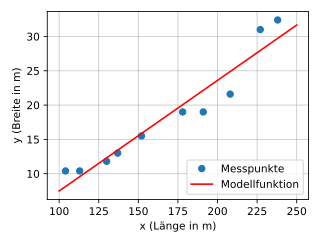
Scatter plot of longitudes and latitudes of ten randomly selected warships with linear balance function plotted.

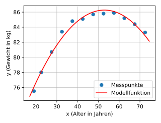
Scatter plot: average weight of men by age with parabolic model function.

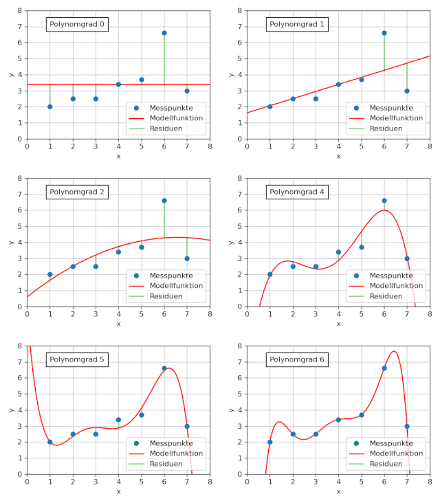
Data set with approximating polynomials

Two-dimensional polynomial surface of second order with 3 × 3 = 9 basis functions:
f(x1, x2) = α $\alpha$ ₀ + α {\displaystyle $\alpha$ 1x11 + α $\alpha$ 2x12 + α $\alpha$ 3x21 + α $\alpha$ 4x11x21 + α $\alpha$ 5x12x21 + α $\alpha$ _6x22 + α $\alpha$ _7x11x22 + α $\alpha$ _8x12x22

Nonlinear model functions

Basic idea and procedure

With the advent of powerful computers, nonlinear regression in particular is gaining in importance. Here, the parameters enter the function nonlinearly. Nonlinear modeling, in principle, allows data to fit any equation of the form $y=f(\alpha )$ . Since these equations define curves, the terms nonlinear regression and curve fitting are most often used interchangeably.

Some nonlinear problems can be transformed into linear ones by suitable substitution and can then be solved as above. A multiplicative model of the form

$y=\alpha _{0}\cdot x^{\alpha _{1}}$

can, for example, be transformed into an additive system by logarithmization. This approach is used, among other things, in growth theory.

In general, nonlinear model functions give rise to a problem of the form

$\min _{\alpha }\|f(\alpha )-y\|_{2},$

with a nonlinear function . Partial differentiation then yields a system of normal equations which can no longer be solved analytically. A numerical solution can be done here iteratively with the Gauss-Newton method.

Current programs often work with a variant, the Levenberg-Marquardt algorithm. Here, the monotonicity of the approximation sequence is guaranteed by a regularization. In addition, the method is more tolerant of larger deviations in the estimated values than the original method. Both methods are related to the Newton method and converge under suitable conditions (the starting point is sufficiently close to the local optimum) mostly quadratically, i.e. the number of correct decimal places doubles in each step.

If differentiation is too costly due to the complexity of the objective function, there are a number of other methods available as fallback solutions that do not require derivatives, see at Methods of local nonlinear optimization.

Example from enzyme kinetics of a non-linearizable model function.

An example of regression models that are fully nonlinear is enzyme kinetics. Here, it is required that "only" (reaction rate) and not α $\alpha$ (substrate concentration) is subject to error and thus α $\alpha$ can be used as a variable. Although the Lineweaver-Burk relation is an algebraically correct transformation of the Michaelis-Menten equation $v=V_{\mathrm {max} }\cdot [S]/(K_{m}+[S])$ , but its application gives correct results only if the measured values are error-free. This results from the fact that reality can only be described with an extended Michaelis-Menten relation

$\nu _{i}={\frac {V_{\max }\left[S_{i}\right]}{K_{m}+\left[S_{i}\right]}}(1+e_{i})\ {\boldsymbol {\nu }}_{i}$

with $e_{i}$ as error parameter. This equation can no longer be linearized, so the solution must be determined iteratively.

Misconduct for failure to comply with the requirements

The method of least squares allows to calculate the most probable of all model parameters under certain conditions. For this purpose, a correct model must have been chosen, a sufficient amount of measured values must be available and the deviations of the measured values compared to the model system must form a normal distribution. In practice, however, the method can be used for various purposes even if these requirements are not met. Nevertheless, it should be noted that the least squares method can produce completely undesirable results under certain unfavorable conditions. For example, there should be no outliers in the measured values, as these distort the estimation result. Moreover, multicollinearity between the parameters to be estimated is unfavorable, since it causes numerical problems. Incidentally, regressors that are far from the others can also strongly influence the results of the equalization calculation. This is referred to as high leverage values.

Multicollinearity

The phenomenon of multicollinearity arises when the measurement series of two given variables $x_{i}$ and $x_{j}$ are very highly correlated, i.e. almost linearly dependent. In the linear case, this means that the determinant of the normal equation matrix $A^{T}A$ very small and the norm of the inverse is conversely very large; thus, the condition of $A^{T}A$ is strongly affected. The normal equations are then difficult to solve numerically. The solution values can become implausibly large, and even small changes in the observations cause large changes in the estimated values.

Outlier

Data values that "do not fit into a measurement series" are defined as outliers. These values strongly influence the calculation of the parameters and falsify the result. To avoid this, the data must be examined for erroneous observations. The detected outliers can, for example, be eliminated from the measurement series or alternative outlier-resistant calculation methods such as weighted regression or the three-group method must be applied.

In the first case, after the first calculation of the estimated values, statistical tests are performed to check whether there are outliers in individual measured values. These measured values are then eliminated and the estimated values are calculated again. This procedure is suitable if there are only a few outliers.

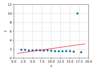
In weighted regression, the dependent variables are weighted depending on their residuals. Outliers, i.e., observations with large residuals, are given a small weight, which may be graded according to the size of the residual. In the Mosteller and Tukey (1977) algorithm, referred to as "biweighting," unproblematic values are weighted by 1 and outliers are weighted by 0, which conditions the suppression of the outlier. Weighted regression usually requires several iterations until the set of detected outliers no longer changes.

Outlier from y: The value pulls the straight line upwards

Generalized least squares models

If one softens the strong requirements in the method for the error terms, one obtains so-called generalized least squares approaches. Important special cases then again have their own names, for example the weighted least squares method (WLS), in which the errors are still assumed to be uncorrelated, but no longer of equal variance. This leads to a problem of the form

$\|D(A\alpha -y)\|_{2},$

where D is a diagonal matrix. If the variances vary strongly, the corresponding normal equations have a very large condition, which is why the problem should be solved directly.

Assuming even further that the errors in the measured data should also be accounted for in the model function, the "total least squares" results are of the form

$\min _{E,r}\|(E,r)\|_{F},(A+E)\alpha =b+r,$

where the error in the model and the error in the data.

Finally, there is the option of not using a normal distribution as a basis. This corresponds, for example, to minimization not in the Euclidean norm, but in the sum norm. Such models are topics of regression analysis.

Questions and Answers

Q: What is least squares?

A: Least squares is a procedure in mathematics that constructs a function from a number of observed values with the idea of minimizing the sum of the squared differences between the observed value and its data point.

Q: What is the basic idea behind the least squares method?

A: The basic idea behind the least squares method is to construct a function that minimizes the sum of the squared differences between the observed value and its data point.

Q: Who developed the least squares method?

A: Carl Friedrich Gauss is credited for developing the method in 1795 and used it to recover the lost asteroid 1 Ceres which he published in 1807. Adrien-Marie Legendre independently developed the same method in 1805.

Q: What was Carl Friedrich Gauss's contribution to the least squares method?

A: Carl Friedrich Gauss developed the least squares method and used it to recover the lost asteroid 1 Ceres.

Q: What was Adrien-Marie Legendre's contribution to the least squares method?

A: Adrien-Marie Legendre developed the same method independently of Gauss in 1805.

Q: How is the difference between observed values and data points calculated in least squares?

A: The difference between observed values and data points is squared, for each value, and then summed to determine the total difference.

Q: What is the objective of least squares?

A: The objective of least squares is to create a function that accurately represents a set of observed values by minimizing the error between the observed values and the predicted values.

Least squares

History

The procedure

Requirements

Minimization of the sum of the squares of the errors

Linear model function

Special case of a simple linear compensation line

Derivation and method

Example with a compensation line

Simple polynomial compensation curves

Special case of a linear balance function with several variables

The general linear case

Solution of the minimization problem

Derivation and method

Numerical treatment of the solution

Problems with constraints

Nonlinear model functions

Basic idea and procedure

Example from enzyme kinetics of a non-linearizable model function.

Misconduct for failure to comply with the requirements

Multicollinearity

Outlier

Generalized least squares models

Questions and Answers

Q: What is least squares?

Q: What is the basic idea behind the least squares method?

Q: Who developed the least squares method?

Q: What was Carl Friedrich Gauss's contribution to the least squares method?

Q: What was Adrien-Marie Legendre's contribution to the least squares method?

Q: How is the difference between observed values and data points calculated in least squares?

Q: What is the objective of least squares?

Search by letter