AlegsaOnline.com

JPEG: lossy image compression standard for photographs and continuous-tone images

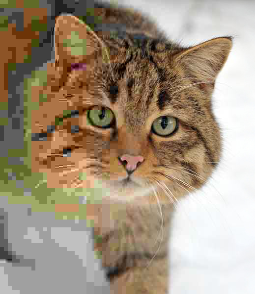
JPEG is a lossy image standard for photographs and continuous-tone images that uses adjustable compression to trade quality for smaller files. Widely supported (.jpg/.jpeg); good for photos, less suited to text or flat-color art.

Author: Leandro Alegsa Creation date: November 13, 2022 Last updated: April 10, 2026

simple.wikipedia.org · CC BY-SA 4.0

The JPEG format is a widely used image file format that stores photographic and other continuous-tone images using adjustable compression. The algorithm allows users to set a balance between image appearance and storage size: higher quality settings preserve more detail and produce larger files, while stronger compression reduces file size at the cost of visible artifacts. JPEG files are extremely common on the World Wide Web and on consumer cameras and mobile devices. The name comes from the Joint Photographic Experts Group, the organization that defined the standard. Many operating systems and applications recognize several file extensions for JPEG images, such as .jpg, .jpeg and .jpe.

How it works

Most JPEG implementations use a lossy compression technique based on the discrete cosine transform; this removes some image information to achieve smaller files.
The degree of compression is selectable, so the same image can be stored with different trade-offs between fidelity and file size. Tools that compress images typically expose a quality slider or compression level.
JPEG is well-suited to photographs and complex color gradients but is less effective for crisp line art, text, or images with large areas of flat color where compression artifacts are more noticeable.

Common characteristics and use

Widespread support: nearly all web browsers, image viewers, printers and digital cameras can read JPEG files.
Variations: the standard includes baseline (progressive) modes and has inspired other JPEG-family formats that target different needs (higher compression efficiency, lossless modes, etc.).
File extensions: users will typically encounter names ending in .jpg, .jpeg or .jpe; historical platform limits led to the shorter .jpg being common on some systems.

Logo

An image with quality levels decreasing from left to right

Overview and standards

The JPEG standard ISO/IEC 10918-1 defines the following modes, of which only the colored ones are in use:

Sequential (Sequential)				Progressive (Progressive)				Lossless	Hierarchical
Huffman coding		Arithmetic coding		Huffman coding		Arithmetic coding
8 bit	12 Bit	8 bit	12 Bit	8 bit	12 Bit	8 bit	12 Bit

In addition to the lossy mode defined in ISO/IEC 10918-1, there is also the improved, lossless compression method JPEG-LS, which was defined in another standard. There is also the JBIG standard for compressing black and white images.

JPEG and JPEG-LS are defined in the following standards:

JPEG (lossy and lossless):		ITU-T T.81 (PDF; 1.1 MB), ISO/IEC IS 10918-1
JPEG (extensions):		ITU-T T.84
JPEG-LS (lossless, enhanced):		ITU-T T.87, ISO/IEC IS 14495-1

The JPEG standard is officially entitled Information technology - Digital compression and coding of continuous-tone still images: Requirements and guidelines. The "Joint" in the name comes from the cooperation of ITU, IEC and ISO.

The JPEG compression

The JPEG standard defines 41 different subfile formats, but usually only one of them is supported (and which also covers almost all use cases).

Compression is achieved by applying several processing steps, four of which are lossy.

Color model conversion from (mostly) RGB color space to YCbCr color model (analogous to CCIR 601). (theoretically lossless, according to CCIR 601 lossy).
Low-pass filtering and subsampling of the color deviation signals Cb and Cr (lossy).
Division into 8×8 blocks and discrete cosine transformation of these blocks (theoretically lossless, but lossy due to rounding errors).
Quantization (lossy).
Rearrangement.
Entropy coding.

Data reduction is achieved by the lossy processing steps in conjunction with entropy coding.

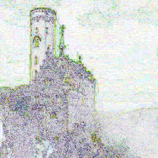
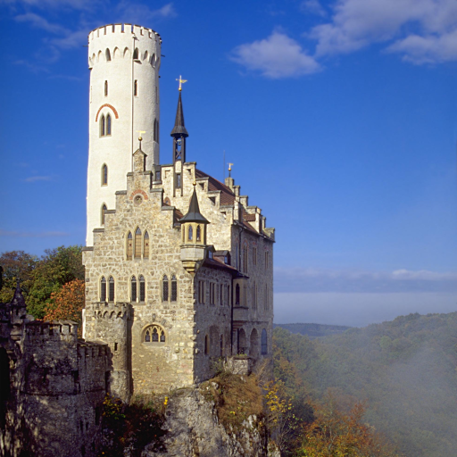
Compressions up to about 1.5-2 bit/pixel are visually lossless, at 0.7-1 bit/pixel good results are still achievable, below 0.3 bit/pixel JPEG becomes practically unusable, the image is increasingly covered by unmistakable compression artefacts (block formation, stepped transitions, colour effects at grey wedges). The successor JPEG 2000 is much less prone to this kind of artifacts.

If you look at 24-bit RGB files as the source format, you get compression rates of 12 to 15 for visually lossless images and up to 35 for still good images. The quality, however, depends on the type of image in addition to the compression rate. Noise and regular fine structures in the image reduce the maximum possible compression rate.

The JPEG Lossless Mode for lossless compression uses a different method (predictive coder and entropy coding).

Color model conversion

The original image, which is usually an RGB image, is converted into the YCbCr color model. Basically, the YPbPr scheme according to CCIR 601 is used:

${\begin{bmatrix}Y'\\Pb\\Pr\end{bmatrix}}\approx {\begin{bmatrix}0{,}299&0{,}587&0{,}114\\-0{,}168736&-0{,}331264&0{,}5\\0{,}5&-0{,}418688&-0{,}081312\end{bmatrix}}\cdot {\begin{bmatrix}R'\\G'\\B'\end{bmatrix}}$

Since the R′G′B′ values are already available digitally as 8-bit numbers in the range {0, 1, ..., 255}, the YPbPr components only need to be shifted (renormalized), resulting in the Y′ (luminance), Cb (color blueness), and Cr (color redness) components:

${\begin{bmatrix}Y'\\Cb\\Cr\end{bmatrix}}\approx {\begin{bmatrix}0\\128\\128\end{bmatrix}}+{\begin{bmatrix}0{,}299&0{,}587&0{,}114\\-0{,}168736&-0{,}331264&0{,}5\\0{,}5&-0{,}418688&-0{,}081312\end{bmatrix}}\cdot {\begin{bmatrix}R'_{d}\\G'_{d}\\B'_{d}\end{bmatrix}}$

The components are now again in the value range {0, 1, ..., 255}.

During the conversion of the color model, the usual rounding errors occur due to limited calculation accuracy and, in addition, a data reduction, since the Cb and Cr values are only calculated for every second pixel (see CCIR 601).

Low-pass filtering of color difference signals

The color deviation signals Cb and Cr are usually stored in reduced resolution. For this purpose they are low-pass filtered and undersampled (in the simplest case by averaging).

Usually, vertical and horizontal subsampling by a factor of 2 each is used (YCbCr 4:2:0), which reduces the amount of data by a factor of 4. This conversion takes advantage of the fact that the spatial resolution of the human eye is significantly lower for colors than for brightness transitions.

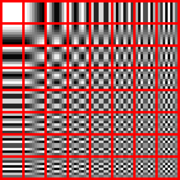
Block formation and discrete cosine transformation

Each component (Y, Cb and Cr) of the image is divided into 8×8 blocks. These are subjected to a two-dimensional discrete cosine transform (DCT):

$F_{xy}={1 \over 4}C_{x}C_{y}\sum _{m=0}^{7}\sum _{n=0}^{7}f_{mn}\cos {\frac {(2m+1)x\pi }{16}}\cos {\frac {(2n+1)y\pi }{16}}$

with

$C_{x},C_{y}={\begin{cases}{1 \over {\sqrt {2}}}&{\text{wenn }}x,y=0\\1&{\text{sonst }}\end{cases}}$

This transform can be implemented using the fast Fourier transform (FFT) with very little effort. The DCT is an orthogonal transform, has good energy compression properties and there is an inverse transform, the IDCT (which also means that the DCT is lossless, no information was lost, as the data was merely converted into a more favorable form for further processing).

Quantization

As with all lossy coding methods, the actual data reduction (and quality degradation) is achieved by quantization. To do this, the DCT coefficients are divided by the quantization matrix (divided element by element) and then rounded to the nearest integer:

$F^{Q}(x,y)=\operatorname {round} \left({\frac {F(x,y)}{Q(x,y)}}\right)$

An irrelevance reduction takes place during this rounding step. The quantization matrix is responsible for both the quality and the compression rate. It is stored in the header of JPEG files (DQT marker).

The quantization matrix is optimal if it approximately represents the sensitivity of the eye for the corresponding spatial frequencies. For coarse structures the eye is more sensitive, therefore the quantization values for these frequencies are smaller than those for high frequencies.

Here is an example of a quantization matrix and its application to an 8×8 block of DCT coefficients:

${\begin{alignedat}{2}Q&={\begin{bmatrix}10&15&25&37&51&66&82&100\\15&19&28&39&52&67&83&101\\25&28&35&45&58&72&88&105\\37&39&45&54&66&79&94&111\\51&52&58&66&76&89&103&119\\66&67&72&79&89&101&114&130\\82&83&88&94&103&114&127&142\\100&101&105&111&119&130&142&156\end{bmatrix}}\\F&={\begin{bmatrix}782{,}91&44{,}93&172{,}52&-35{,}28&-20{,}58&35{,}93&2{,}88&-3{,}85\\-122{,}35&-75{,}46&-7{,}52&55{,}00&30{,}72&-17{,}73&8{,}29&1{,}97\\-2{,}99&-32{,}77&-57{,}18&-30{,}07&1{,}76&17{,}63&12{,}23&-13{,}57\\-7{,}98&0{,}66&2{,}41&-21{,}28&-31{,}07&-17{,}20&-9{,}68&16{,}94\\3{,}87&7{,}07&0{,}56&5{,}13&-2{,}47&-15{,}09&-17{,}70&-3{,}76\\-3{,}77&0{,}80&-1{,}46&-3{,}50&1{,}48&4{,}13&-6{,}32&-18{,}47\\1{,}78&3{,}28&4{,}63&3{,}27&2{,}39&-2{,}31&5{,}21&11{,}77\\-1{,}75&0{,}43&-2{,}72&-3{,}05&3{,}95&-1{,}83&1{,}98&3{,}87\end{bmatrix}}\\F^{Q}&={\begin{bmatrix}78&3&7&-1&0&1&0&0\\-8&-4&0&1&1&0&0&0\\0&-1&-2&-1&0&0&0&0\\0&0&0&0&0&0&0&0\\0&0&0&0&0&0&0&0\\0&0&0&0&0&0&0&0\\0&0&0&0&0&0&0&0\\0&0&0&0&0&0&0&0\end{bmatrix}}\end{alignedat}}$

where $F^{Q}$ is calculated with:

$F^{Q}(0,0)=\operatorname {round} \left({\frac {F(0,0)}{Q(0,0)}}\right)=\operatorname {round} \left({\frac {782{,}91}{10}}\right)=78$

$F^{Q}(0,1)=\operatorname {round} \left({\frac {F(0,1)}{Q(0,1)}}\right)=\operatorname {round} \left({\frac {-122{,}35}{15}}\right)=-8$

etc.

Reordering and differential coding of the DC component

The 64 coefficients of the discrete cosine transformation are sorted by frequency. This results in a zigzag order, starting with the DC component with the frequency 0. After the English Direct Current (for direct current), it is abbreviated DC, here it denotes the average brightness. The coefficients with a high value are now usually placed first and small coefficients further back. This optimizes the input of the following runlength coding. The reordering sequence looks like this:

1 2 6 7 15 16 28 29 3 5 8 14 17 27 30 43 4 9 13 18 26 31 42 44 10 12 19 25 32 41 45 54 11 20 24 33 40 46 53 55 21 23 34 39 47 52 56 61 22 35 38 48 51 57 60 62 36 37 49 50 58 59 63 64

Furthermore, the DC part is coded again differentially to the block to the left of it and in this way the dependencies between adjacent blocks are taken into account.

The above example leads to the following rearranged coefficients

119 … 78 3 -8 0 -4 7 -1 0 -1 0 0 0 -2 1 0 1 1 -1 0 … 102 5 -5 0 3 -4 2 -1 0 0 0 0 1 1 -1 0 0 -1 0 0 0 0 0 0 0 1 0 … 75 -19 2 -1 0 -1 1 -1 0 0 0 0 0 0 1 … 132 -3 -1 -1 -1 0 0 0 -1 0 …

Differential coding of the first coefficient then gives:

-41 3 -8 0 -4 7 -1 0 -1 0 0 0 -2 1 0 1 1 -1 0 … 24 5 -5 0 3 -4 2 -1 0 0 0 0 1 1 -1 0 0 -1 0 0 0 0 0 0 0 1 0 … -27 -19 2 -1 0 -1 1 -1 0 0 0 0 0 0 1 … 57 -3 -1 -1 -1 0 0 0 -1 0 …

In regions with little structure (of the same image), the coefficients can also look like this:

35 -2 0 0 0 1 0 … 4 0 1 0 … 0 0 2 0 1 0 … -13 0 -1 … 8 1 0 … -2 0 …

These areas can of course be coded better than areas rich in structure. For example, by means of run-length coding.

Zigzag re-sorting of DCT coefficients does fall within the scope of protection of US patent 4,698,672 (and other applications and patents in Europe and Japan). However, it was found in 2002 that the claimed prior art process was not novel, so the claims would have been unlikely to be enforceable. In the meantime, the patents from the patent family relating to the aforementioned US patent have also lapsed due to the passage of time, such as EP patent 0 266 049 B1 in September 2007.

Entropy coding

A Huffman encoding is usually used as the entropy encoding. The JPEG standard also allows arithmetic coding. Although this generates files that are between 5 and 15 percent smaller, it is hardly ever used for patent reasons, and this encoding is also significantly slower.