Interval arithmetic: verified numerical computation and error bounding
An introduction to interval arithmetic: definitions, basic operations, extensions, uses for error bounding and verified computing, and key limitations including overestimation and dependency issues.
Interval arithmetic is a numerical framework that represents uncertain or imprecise real values by closed intervals [a, b] instead of single numbers. Each interval is understood to contain the true, but possibly unknown, value. Arithmetic and functions are extended so that every result is itself an interval that provably contains all possible outcomes produced by picking one number from each input interval. This inclusion property makes interval arithmetic useful for reliable error bounds, automated detection of rounding and modelling errors, and for producing guaranteed enclosures of solutions in scientific computation. For background on computational contexts where intervals are used, see computational arithmetic resources.
Image gallery
10 Images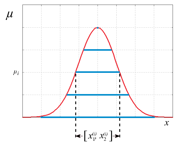


Basic operations and properties
Elementary operations are defined so the result covers all combinations of endpoints. For example, addition is [a,b]+[c,d] = [a+c, b+d]; subtraction is [a,b]-[c,d] = [a-d, b-c]. Multiplication and division require examining multiple endpoint products and, for division, additional care when the divisor interval contains zero. Implementations typically use directed rounding (outward rounding) so that floating-point endpoints are adjusted to guarantee containment despite rounding. A simple demonstration appears in many introductions: [1,2] + [3,4] = [4,6]. Interval functions are built from these operations or by taking the range of a function over an interval; one standard construction is the natural interval extension, which substitutes interval arguments into an expression and evaluates with interval arithmetic.
Representations and extensions
Interval arithmetic comes in several flavors: classical real intervals, affine forms and modal intervals are examples of richer representations that attempt to reduce overestimation and capture dependency between quantities. Interval matrices and interval systems of linear equations extend the idea to linear algebra. Software libraries implement these concepts for many programming languages; they typically provide basic interval types, elementary functions, and often algorithms for root finding and global optimization. For introductions to libraries and implementation strategies, consult interval documentation and practical guides such as error analysis tutorials.
Applications and examples
Interval arithmetic is widely used where guaranteed bounds are required. Typical applications include validated numerics (producing mathematically rigorous error bounds for computed quantities), propagation of measurement uncertainty (each measurement interval captures instrument error), robust control and verification of numerical algorithms, and global optimization where intervals help enclose minima or roots. Simple use-cases include computing bounds on a function given uncertain inputs, or verifying that no root exists in a region. For practical case studies and sample code, see worked examples and implementation notes at practical guides.
Limitations and notable facts
Despite its strengths, interval arithmetic has limitations. The dependency problem leads to overestimation: evaluating the same variable multiple times in an expression can produce unnecessarily wide intervals. For instance, x-x evaluated with x=[1,2] yields [1-2,2-1] = [-1,1] instead of the exact {0}. Specialized techniques—such as algebraic reformulation, domain splitting, or using affine arithmetic—help to mitigate this issue. Another practical concern is performance: guaranteed containment requires conservative rounding and sometimes additional computations, which can be slower than conventional floating-point arithmetic.
History and practical considerations
The modern systematic study of interval methods dates to mid-20th century numerical analysis, with further formalization in the work of researchers like R. E. Moore and others who developed the theoretical foundations and algorithms. Today interval techniques form a core tool in validated computing and appear in many scientific and engineering toolkits. When adopting interval arithmetic, practitioners must balance the need for rigorous bounds against increased computational cost and potential over-conservatism. For further reading and authoritative surveys, consult accessible overviews at further reading.
- Key idea: represent uncertainty by intervals and propagate them through computations to maintain proven bounds.
- Practical tip: transform expressions and split domains to reduce overestimation.
- Caveat: division by intervals containing zero is undefined and must be treated specially.


Patents
One of the major promoters of interval arithmetic, G. William Walster of Sun Microsystems, filed several patents in the field of interval arithmetic with the U.S. Patent and Trademark Office in 2003/04, partly together with Ramon E. Moore and Eldon R. Hansen. However, the validity of these claims is highly disputed in the interval arithmetic research community, as they may merely reflect prior art.
Implementations
There are many software packages that allow the development of numerical applications using interval arithmetic. These are usually implemented in the form of programme libraries. However, there are also C++ and Fortran translators that have interval data types and correspondingly suitable operations as language extensions, so that interval arithmetic is directly supported.
Since 1967, XSC extensions for scientific computation have been developed for various programming languages, including C++, Fortran and Pascal, initially at the University of Karlsruhe. The initial platform was a Zuse Z 23, for which a new interval data type with corresponding elementary operators was made available.
In 1976, Pascal-SC followed, a Pascal variant on a Zilog Z80 that made it possible to quickly create complex routines for automated result verification. This was followed by the Fortran 77-based ACRITH-XSC for the System/370 architecture, which was later also delivered by IBM. From 1991, Pascal-XSC can then be used to generate code for C compilers, and a year later the C++ class library C-XSC already supports many different computer systems. In 1997, all XSC variants were placed under the General Public License and were thus freely available. At the beginning of the 2000s, C-XSC 2.0 was redesigned under the leadership of the Working Group for Scientific Computing at the University of Wuppertal in order to better comply with the C++ standard that had been adopted in the meantime.
Another C++ class library is the Profile/BIAS ("Programmer's Runtime Optimised Fast Interval Library, Basic Interval Arithmetic") created in 1993 at the TU Hamburg-Harburg, which provides the usual interval operations in a user-friendly way. Special emphasis was placed on efficient utilisation of the hardware, portability and independence from a special interval representation.
The Boost collection of C++ libraries also contains a template class for intervals. Its authors are currently trying to get interval arithmetic included in the C++ language standard.
Today, the common computer algebra systems, such as Mathematica, Maple and MuPAD, can also handle intervals. There is also the extension INTLAB for Matlab, which builds on BLAS routines, as well as the toolbox b4m, which provides a profile/BIAS interface.
IEEE Standard 1788-2015
An IEEE standard for interval arithmetic was published in June 2015. There are two free reference implementations developed by members of the working group: The libieeep1788 library for C++ and the interval package for GNU Octave.
A simplified version of the standard is still being developed. This should be even easier to implement and ensure faster dissemination.
Conferences and workshops
Several international conferences and workshops are held annually around the world. The most important conference is SCAN (International Symposium on Scientific Computing, Computer Arithmetic, and Verified Numerical Computation). There are also SWIM (Small Workshop on Interval Methods), PPAM (International Conference on Parallel Processing and Applied Mathematics) and REC (International Workshop on Reliable Engineering Computing).
See also
- Automatic differentiation
- Multigrid method
- Monte Carlo simulation
- Uncertainty of measurement
- INTLAB
Related articles
Author
AlegsaOnline.com Interval arithmetic: verified numerical computation and error bounding Leandro Alegsa
URL: https://en.alegsaonline.com/art/47844
Sources
- link.springer.com : Scientific Computing, Computer Arithmetic, and Validated Numerics 16th International Symposium, SCAN 2014, Würzburg, Germany, September 21-26, 2014. Revised Selected Papers.
- proceedings.com : 13th GAMM-IMACS International Symposium on Scientific Computing, Computer Arithmetic and Verified Numerical Computations (SCAN'2008), Proceedings of a meeting held 29 September - 3 October 2008, El Paso, Texas, USA. Special volume devoted to materials presented at SCAN 2012. Published by the Institute of Computational Technologies
- proceedings.com : 12th GAMM-IMACS International Symposium on Scientific Computing, Computer Arithmetic and Validated Numerics (SCAN 2006), Proceedings of a meeting held 26-29 September 2006, Duisburg, Germany. Published by the Institute of Electrical and Electronics Engineers