Fourier Transform: Definition, Properties, History and Applications
Comprehensive overview of the Fourier transform: its definition, intuition, principal properties, historical development, computation (DFT/FFT) and common applications in science and engineering.
Overview
The Fourier transform is a fundamental mathematical operation that decomposes a function or signal into its constituent frequencies. Rather than viewing a signal only as a function of time or space, the transform represents the same information as a distribution over frequency, revealing periodic components, spectral energy, and phase relationships. This frequency-domain perspective clarifies behaviors that are hard to see in the original domain, and it underpins many techniques in analysis, signal processing, physics, and engineering. For a concise technical description see mathematical transform.
Image gallery
3 Images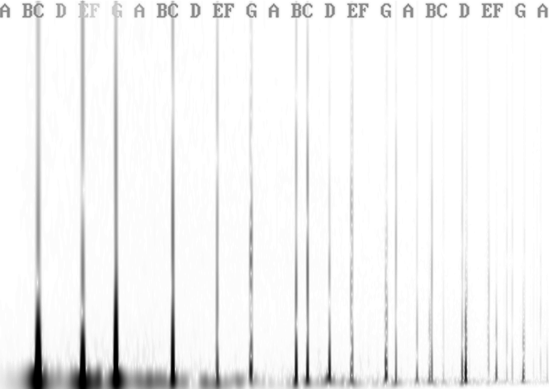

Definition and basic formula
For a suitably well-behaved function f(x), the continuous Fourier transform F(α) can be written in one common convention as F(α) = ∫_{-∞}^{+∞} f(x) e^{-2π i α x} dx, where α denotes frequency and i is the imaginary unit. The inverse transform reconstructs f from F via f(x) = ∫_{-∞}^{+∞} F(α) e^{+2π i α x} dα. These integrals use complex exponentials to project the input onto sinusoidal components; the magnitude |F(α)| indicates how much of frequency α is present and the argument (phase) encodes its phase shift. See a basic introduction at frequency decomposition and a typical visualization at frequency spectrum.
Interpretation and core properties
Intuitively, the Fourier transform measures overlap between the input signal and sinusoids of varying frequency. Peaks in the transform correspond to dominant sinusoidal components; a pure tone yields a sharp spike, while noise produces a broad background. Several algebraic and analytic properties make the transform especially useful: linearity, time and frequency shifting, scaling, modulation, and the convolution theorem, which turns convolution in one domain into multiplication in the other. These properties are often collected in reference tables; for illustration and derivations consult property list.
Because the transform uses complex exponentials, understanding results requires familiarity with complex numbers and integrals; introductory material on complex analysis and integration is available at imaginary numbers and integration. The transform can be applied to real signals (yielding symmetric spectra) and to complex-valued functions in general.
Historical background
The idea that arbitrary functions can be represented by sums of sinusoids traces back to the work of Joseph Fourier in the early 19th century, initially motivated by heat conduction problems. Fourier introduced trigonometric series to represent temperature distributions; later mathematicians and physicists formalized convergence and developed the modern integral transform. Subsequent developments connected the formalism to complex analysis, distribution theory, and functional analysis; for historical notes see historical overview and further reading at mathematical history.
Applications and examples
The Fourier transform appears across science and technology. In audio processing it separates musical notes and noise from time-domain recordings, enabling filtering, compression and pitch detection; see an accessible example at sound analysis. In imaging and radiology it supports reconstruction of images from projection data (as in MRI and CT), with clinical importance described at radiology applications. In oceanography and geophysics it helps identify periodic phenomena and waves (oceanography), while in quantum mechanics the transform links position and momentum representations of wavefunctions. Modern machine learning and data analysis often use spectral methods for feature extraction and kernel design; introductory resources are available at machine learning. Other applied areas include cryptography, communications, and vibration analysis (cryptography, visualization).
An elementary auditory example: a chord consisting of three musical notes produces a time-domain waveform whose Fourier transform shows three peaks at the corresponding frequencies. Plotting frequency (x-axis) versus amplitude (y-axis) yields a spectrum that directly exposes those notes and their relative strengths; interactive demonstrations and plots are widely available at sine and cosine decomposition.
Computation: discrete transforms and algorithms
Practical computation uses discrete versions of the transform. The Discrete Fourier Transform (DFT) converts a finite sequence of samples to a sampled frequency spectrum, and the Fast Fourier Transform (FFT) is an efficient algorithm to compute the DFT in O(N log N) operations. These methods make spectral analysis feasible for large data sets and real-time applications. Software libraries implement many variants and optimizations; see algorithmic introductions at phases and amplitudes and practical guides.
Common numerical concerns include sampling, aliasing, windowing, and numerical precision. The Nyquist–Shannon sampling theorem states that bandlimited signals sampled above twice their highest frequency can be reconstructed exactly from samples; failure to meet sampling criteria produces aliasing artifacts. Window functions reduce spectral leakage at the cost of broadening peaks. For practical tutorials consult complex plane and graphing examples.
Variants, distinctions and notable points
There are multiple Fourier-related transforms and normalizations: the continuous Fourier transform, the inverse transform, the DFT, the discrete-time Fourier transform (DTFT) for sampled but infinite sequences, and multidimensional transforms for images. The choice of normalization factor (where 2π appears) varies between fields; care is required when comparing formulas. Spectral methods extend to generalized functions (distributions) and to non-periodic or non-stationary signals via short-time and wavelet transforms when local frequency content matters. For focused comparisons see overview and integration background.
Finally, the Fourier transform remains a central analytical tool because it translates differential equations into algebraic ones, simplifies linear systems analysis, and reveals hidden regularities. Its broad reach—from pure mathematics to practical engineering—explains why it is taught across many disciplines and implemented in virtually every scientific computing environment. For application examples and reference material visit spectral plots and foundational concepts.


Questions and answers
Q: What is the Fourier transform?
A: The Fourier transform is a mathematical function that can be used to find the base frequencies that a wave is made of. It takes a complex wave and finds the frequencies that make it up, allowing it to identify the notes that make up a chord.
Q: What are some uses of the Fourier transform?
A: The Fourier transform has many uses in cryptography, oceanography, machine learning, radiology, quantum physics as well as sound design and visualization.
Q: How is the Fourier transform calculated?
A: The Fourier transform of a function f(x) is given by F(α) = ∫−∞+∞f(x)e−2πiαxdx where α is a frequency. This returns a value representing how prevalent frequency α is in the original signal. The inverse Fourier transform is given by f(x) = ∫−∞+∞F(α)e+2πixαdα.
Q: What does an output of a Fourier Transform look like?
A: An output of a Fourier Transform can be called either a frequency spectrum or distribution because it displays a distribution of possible frequencies of the input.
Q: How do computers calculate Fast Fourier Transforms?
A: Computers use an algorithm called Fast Fourier Transform (FFT) to quickly calculate any but the simplest signals' transforms.
Q: What does looking at signals with respect to time not show us?
A: Looking at signals with respect to time does not make it obvious what notes are present in them; many signals make more sense when their frequencies are separated and analyzed individually instead.
Related articles
Author
AlegsaOnline.com Fourier Transform: Definition, Properties, History and Applications Leandro Alegsa
URL: https://en.alegsaonline.com/art/35911