
Exponential distribution
Continuous probability distribution on nonnegative reals with density f(x)=λ e^{-λx}. Models interarrival times in Poisson processes; memoryless property; mean 1/λ and variance 1/λ^2. Special case of gamma and Weibull.
Overview
The exponential distribution is a continuous probability model supported on the nonnegative axis. It describes the time until a single event occurs when events happen independently at a constant average rate. Common notation is Exp(λ), where the parameter λ (lambda) is the rate. The distribution has probability density function PDF: f(x) = λ e^{-λ x} for x ≥ 0 and cumulative distribution function CDF: F(x) = 1 − e^{-λ x}.
Image gallery
3 Images


Basic properties
Key numerical characteristics are simple: the expected value (mean) is 1/λ and the variance is 1/λ². The exponential is memoryless, meaning that for any s, t ≥ 0, P(X > s + t | X > s) = P(X > t). This is the only continuous distribution with that property. The model can also be expressed using a scale parameter θ = 1/λ instead of the rate.
Connections and special cases
The exponential distribution is the continuous analogue of the geometric distribution and arises naturally as the distribution of interarrival times in a Poisson process. It is a special case of the gamma distribution with shape parameter 1, and of the Weibull distribution with shape parameter 1. These relationships make the exponential a useful building block in probability and statistics.
Uses and examples
Applied settings that often use an exponential model include queueing and service systems, reliability engineering, and survival analysis. Examples: the time between arrivals of customers in a simple Poisson arrival model, the lifetime of a component whose failure rate is constant over time, or the waiting time until the next radioactive decay event (under ideal assumptions).
Notes, limitations and alternatives
- The constant hazard (failure) rate implied by the exponential is a strong assumption and may not hold for many real systems. If the hazard varies with time, alternatives such as the Weibull or generalized gamma distributions are more flexible.
- Parameter estimation is straightforward: for independent noncensored observations, the maximum likelihood estimator of λ is the reciprocal of the sample mean.
- Because of its memoryless property, the exponential is frequently used for analytic models where tractability is important, even when it is only an approximation to observed data.
Further reading
Introductory sources on continuous distributions discuss the exponential as a fundamental law for modeling random time intervals. For formal definitions and proofs of properties such as memorylessness and connections to the Poisson process, see standard probability texts or online references labeled as positive or real numbers in measure-theoretic treatments.

Definition
A continuous random variable  satisfies the exponential distribution
  with the positive real inverse scale parameter λ
 , if they have the density function
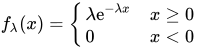
has. If a random variable has this density, then one also writes  or
or  .
.
The parameter λ  has the character of an event rate and
  that of an event distance (mean range or mean lifetime).
An alternative parameterization (common especially in Anglo-Saxon countries) leads to the density function
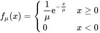 .
.
The relation to the above parametrization is simply μ  . To avoid misunderstandings, it is recommended to state the expected value explicitly, i.e. to speak of an exponential distribution with expected value .
Relationship to other distributions
Relationship to the continuous uniform distribution
If a continuous random variable uniformly ![[0,1]](https://www.alegsaonline.com/image/738f7d23bb2d9642bab520020873cccbef49768d.svg) distributed on the interval , then
distributed on the interval , then 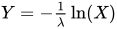 satisfies the exponential distribution with parameter λ .
Relationship to normal distribution
If the random variables and are  standard normally distributed and independent, then
  is exponentially distributed with parameter λ
  .
.
Relationship to geometric distribution
In analogy to the discrete geometric distribution, the continuous exponential distribution determines the waiting time until the first occurrence of an event that occurs according to a Poisson process; thus, the geometric distribution can be considered as a discrete equivalent of the exponential distribution.
Relationship to gamma distribution
- The generalization of the exponential distribution, i.e. the waiting time until the arrival of the
 -th event of a Poisson process, is described by the gamma distribution. Thus, the exponential distribution with parameter λ is identical to the gamma distribution with parameters
  and λ . Accordingly, the exponential distribution also has all the properties of the gamma distribution. In particular, the sum of independent, -distributed random variables is gamma or Erlang distributed with parameters and λ .
- Convolving two exponential distributions with the same λ yields a gamma distribution with
 ,
,  .
.
Relationship to gamma-gamma distribution
If the parameter λ of the exponential distribution a random variable distributed like a gamma distribution  , then the resulting random variable is
  distributed like a gamma-gamma distribution .
Relationship to the Pareto distribution
If is Pareto distributed  with parameters λ and then is
  exponentially distributed with parameter λ .
Relationship to the Poisson distribution
The distances between the occurrence of random events can often be described by the exponential distribution. In particular, it holds that the distance between two consecutive events of a Poisson process with rate λ is exponentially distributed with parameter λ . In this case, the number of events in an interval of length Δ is  Poisson distributed with parameter λ
  .
.
Derivation: Let w be a location or time variable and λ the small constant occurrence frequency of events in the unit interval of w . Then, using Poisson's assumptions, find the probability of the next occurrence of an event in the small interval ![[w,w+\Delta w]](https://www.alegsaonline.com/image/27b2040fcb6fda995a889b38b998fc103ffa422e.svg) as the product of the probability of having no event up to w and one in the interval :
as the product of the probability of having no event up to w and one in the interval :

From this, after dividing by Δ the probability density 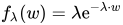 of the exponential distribution with λ as event rate and as mean event distance.
Relationship to the Erlang distribution
- For a Poisson process, the random number of events up to a defined time is determined by means of Poisson distribution, the random time up to the -th event is Erlang distributed. In the case
 , this Erlang distribution transitions to an exponential distribution
  , which can be used to determine the time to the first random event and the time between two consecutive events.
- The sum of independent exponentially distributed random variables has the Erlang distribution -th order
 .
.
Relationship to Weibull distribution
- With β
 , the Weibull distribution transitions to the exponential distribution. In other words, the exponential distribution handles problems with constant failure rate λ . However, if one examines problems with increasing (
  ) or decreasing (
  ) failure rate, then one transitions from the exponential distribution to the Weibull distribution.
 - If is exponentially distributed, then
 Weibull distributed.
Relationship to the chi-square distribution
The chi-squared distribution transitions to the exponential distribution for  with parameter λ
Relationship to the Rayleigh distribution
If is exponentially distributed with rate λ , then is  Rayleigh distributed with scale parameter
  .
.
Relationship to the Laplace distribution
If are  two independent random variables, both exponentially distributed to parameter λ , then both
  and
and  Laplace distributed.
Relationship to the standard Gumbel minimum distribution
The density of the logarithm of a standard exponentially distributed random variable  follows a standard Gumbel distribution (minimum)
 .
.
Related articles
Author
AlegsaOnline.com Exponential distribution Leandro Alegsa
URL: https://en.alegsaonline.com/art/32992