AlegsaOnline.com

Differential calculus: rates of change, derivatives, and applications

Differential calculus studies instantaneous rates of change and tangent behavior of functions. It defines derivatives, basic computation rules, higher derivatives, multivariable extensions, and common applications.

Author: Leandro Alegsa Creation date: November 13, 2022 Last updated: May 10, 2026

en.wikipedia.org · CC BY-SA 4.0

Differential calculus is the branch of mathematical analysis concerned with how quantities change in relation to one another. It formalizes the notion of instantaneous rate of change through the derivative and gives a geometric interpretation as the slope of the tangent line to a curve. For general context, see calculus; for the idea of a dependent quantity use variable; and many models are expressed by a function.

Core concepts

The primary object is the derivative. Informally, the derivative of y = f(x) at x=a measures how much y changes per small change in x near a. A common formulation is as a limiting ratio: the derivative is the limit of the difference quotient as the increment approaches zero. A function with a derivative at a point is called differentiable there; differentiability implies continuity, but a continuous function need not be differentiable.

Difference quotient: (f(x+h)-f(x))/h, h→0.
Limit process: taking the limit of the difference quotient defines the derivative.
Basic rules: linearity, product rule, quotient rule, and chain rule simplify calculations.

Notation and higher derivatives

Common notations include f'(x), dy/dx, Df(x) and higher-order derivatives such as f''(x) or d2y/dx2. Higher derivatives describe rates of change of rates of change: for example, acceleration is the second derivative of position with respect to time. The existence and continuity of higher derivatives are central to Taylor series and many approximation methods.

Multivariable extensions

When functions depend on several variables, partial derivatives measure change with respect to one variable while holding others fixed. The gradient is a vector of first partial derivatives and points in the direction of steepest increase. The Jacobian matrix generalizes the derivative for vector-valued functions, and the Hessian matrix collects second partial derivatives to analyze curvature and extrema in multiple dimensions.

Techniques for finding derivatives

Routine computation uses derivative rules and known derivatives of elementary functions. Additional techniques include implicit differentiation for relations not given as explicit functions, logarithmic differentiation for products and powers, and differentiation under the integral sign in certain advanced contexts. When analytic forms are difficult or unavailable, numerical differentiation approximates derivatives from sampled data.

Practical applications

Derivatives appear across science, engineering, and economics. In physics, velocity and acceleration are first and second derivatives of position with respect to time. In optimization, setting derivatives (or gradients) to zero locates candidate maxima and minima; second-derivative tests help classify them. In engineering and control theory, derivatives are used to model rates, sensitivities and linear approximations. In economics, marginal concepts are derivatives of cost, revenue or utility functions.

Historical notes and further study

The development of differential calculus in the late 17th century involved independent contributions by Sir Isaac Newton and Gottfried Wilhelm Leibniz. Newton applied rate-of-change ideas to motion and physical problems; Leibniz developed much of the symbolic notation still used today. See short biographies at Sir Isaac Newton and Gottfried Leibniz. Modern study moves from single-variable theory to multivariable analysis, differential equations and numerical methods, and connects tightly with integral calculus via the fundamental theorem that links differentiation and integration.

Graph of a function (blue) and a tangent to the graph (red). The slope of the tangent is the derivative of the function at the marked point.

Introduction

Introduction by means of an example

If a car is driving on a road, this fact can be used to create a table in which the distance covered since the start of the recording is entered at each point in time. In practice, it is useful not to keep such a table too close-meshed, i.e., for example, to make a new entry only every 3 seconds in a period of 1 minute, which would require only 20 measurements. However, such a table can theoretically be made arbitrarily close-meshed, if every point in time is to be taken into account. In this case, the previously discrete data, i.e. data with a distance, merge into a continuum. The present is then interpreted as a point in time, i.e. as an infinitely short period of time. At the same time, however, the car has covered a theoretically measurable exact distance at every point in time, and if it does not slow down to a standstill or even reverse, the distance will increase continuously, i.e. it will never be the same at any point in time as at another.

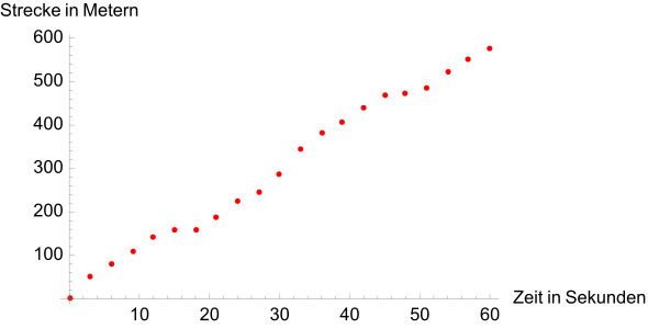
Exemplary representation of a table, every 3 seconds a new measurement is entered. Under such conditions, only average velocities can be calculated in the periods 0 to 3, 3 to 6 etc. seconds can be calculated. Since the distance covered always increases, the car seems to move only forward.

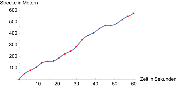
Potential transition to an arbitrarily close-meshed table, which takes the form of a curve after all points have been entered. Now a distance
is assigned to each time point between 0 and 60 seconds. Regions, within which the curve runs more steeply upwards, correspond to time periods, in which a larger number of meters per time unit is covered. In regions with an almost constant number of meters, for example in the range 15-20 seconds, the car drives slowly and the curve runs flat.

The motivation behind the notion of deriving a time-distance table or function is to now be able to specify how fast the car is moving at a certain present time. From a time-stretch table the appropriate time-speed table is to be derived. The background is that speed is a measure of how much the distance traveled changes over time. If the speed is high, a strong increase in the distance can be seen, while a low speed leads to little change. Since each time point has also been assigned a distance, such an analysis should in principle be possible, because with the knowledge of the distance traveled within a time period the following applies to the velocity

$v={\frac {s}{t}}.$

Thus, if $t_{0}$ and $t_{1}$ two different times, "the speed" of the car in the period between them is

$v={\frac {s(t_{1})-s(t_{0})}{t_{1}-t_{0}}}.$

The differences in numerator and denominator have to be formed, since one is only interested in the distance $s(t_{1})-s(t_{0})$ $t_{1}-t_{0}$ traveled within a certain time period Nevertheless, this approach does not provide a complete picture, since initially only velocities for "real time periods" were measured. A present velocity, comparable to a speed camera photo, on the other hand, would refer to an infinitely short time interval. Furthermore, it is very possible that the car still changes its speed even in very short intervals, for example during emergency braking. Accordingly, the upper term "speed" is not applicable and must be replaced by "average speed". Thus, if real time intervals, i.e. discrete data, are used, the model is simplified in that a constant speed is assumed for the car within the intervals considered.

If, on the other hand, we want to move on to a "perfectly fitting" time-velocity table, the term "average velocity in a time interval" must be replaced by "velocity at a point in time". To do this, a time $t_{0}$ must first be chosen. The idea now is to run "real time intervals" in a limit process against an infinitely short time interval and study what happens to the average velocities involved. Although the denominator $t_{1}-t_{0}$ to 0, this is not a problem, because the car can move less and less far in shorter time intervals with a continuous course, i.e. without teleportation, so that numerator and denominator decrease at the same time, and in the limit process an indefinite term " ${\tfrac {0}{0}}$ " arises. This can make sense as a limit value under certain circumstances, for example, express

${\frac {5\,\,\mathrm {Meter} }{\mathrm {Sekunde} }}\,\,\,{\text{und}}\,\,\,{\frac {5\,\,\mathrm {Millimeter} }{\mathrm {Millisekunde} }}\,\,\,{\text{und}}\,\,\,{\frac {5\,\,\mathrm {Nanometer} }{\mathrm {Nanosekunde} }}\,\,\,{\text{usw.}}$

exactly the same velocities. Now there are two possibilities when studying the velocities. Either, they do not show any tendency to approach a certain finite value in the considered limit process. In this case, no velocity valid at time $t_{0}$ can be assigned to the motion of the car, i.e., the term " ${\tfrac {0}{0}}$ " has no definite meaning here. If, on the other hand, there is an increasing stabilization in the direction of a fixed value, then there exists the limit

${\frac {\mathrm {d} s}{\mathrm {d} t}}(t_{0}):=\lim _{t_{1}\to t_{0}}{\frac {s(t_{1})-s(t_{0})}{t_{1}-t_{0}}}=\lim _{h\to 0}{\frac {s(t_{0}+h)-s(t_{0})}{h}}$

and expresses exactly the $t_{0}$ prevailing speed of the car at time The indeterminate term " ${\tfrac {0}{0}}$ " takes on a unique value in this case. The resulting numerical value is also called the derivative of at location $t_{0}$ and the symbol often $s'(t_{0})$ used for it.

The principle of differential calculus

The example of the last section is particularly simple if the increase of the distance of the car with time is uniform, i.e. linear. In this case, one also speaks of a proportionality between time and distance, if at the beginning of the recording ( t=0 ) no distance has been covered yet ( $s(0)=0$ ). This results in an always constant change of the distance in a certain time interval, no matter from when the measurement starts. For example, between 0 and 1 the car covers the same distance as between 9 and 10 seconds. If we assume that the car moves 2 meters further for every second that elapses, proportionality means that it moves only 1 meter for every half second, and so on. In general, then, $s(t)=2t$ i.e., for each additional unit of time, two additional units of distance are added, so that the rate of change at each point is 2 "meters per (added) second".

For the more general case, replacing 2 by any number , i.e. $s(t)=mt$ , then for each elapsed time unit, another distance units are added. This can be seen quickly, because the following applies to the distance difference

$s(t+1)-s(t)=m\cdot (t+1)-mt=mt+m-mt=m.$

In general, the car moves forward in $t_{0}$ time units by a total of $mt_{0}$ distance units - its speed is therefore, in case of the choice of meters and seconds made, constant " meters per second". If the starting value is not $s(0)=0$ but $s(0)=c$ , this does not change anything, since the constant in the upper difference always subtracts out. This is also reasonable from an illustrative point of view: The starting position of the car should be irrelevant for its speed if the motion is uniform.

It can therefore be stated:

Linear functions. For linear functions (note that it does not have to be an origin line), the derivative term is explained as follows. If the function under consideration has the form $f(x)=mx+c$ then the instantaneous rate of change at each point has the value , so it is true for the corresponding derivative function $f'(x)=m$ . Thus, the derivative can be read directly from the data $mx+c$ In particular, every constant function has the derivative , since changing the input values does not change the output value. The measure of change is therefore 0 everywhere.

Sometimes it can be much more difficult if a movement is not uniform. In this case, the course of the time-stretch function may look completely different from a straight line. From the nature of the time-stretch function, it can then be seen that the car's motion trajectories are very varied, which may have to do with traffic lights, curves, traffic jams and other road users, for example. Since such types of progressions are particularly common in practice, it is convenient to extend the derivation notion to non-linear functions as well. Here, however, one quickly encounters the problem that, at first glance, there is no clear proportionality factor that precisely expresses the local rate of change. Therefore, the only possible strategy is to linearize the nonlinear function to reduce the problem to the simple case of a linear function. This technique of linearization forms the very calculus of differential calculus and is of very great importance in calculus, since it helps to reduce complicated processes locally to very easily understood processes, namely linear processes.

The strategy can be exemplified by the non-linear function $f(x)=x^{2}$ The following table shows the linearization of the quadratic function $f(x)=x^{2}$ at position 1.

	0,5	0,75	0,99	0,999	1	1,001	1,01	1,1	2	3	4	100
$x^{2}$	0,25	0,5625	0,9801	0,998001	1	1,002001	1,0201	1,21	4	9	16	10000
	0	0,5	0,98	0,998	1	1,002	1,02	1,2	3	5	7	199

That the linearization is only a local phenomenon is shown by the increasing deviation of the function values at more distant input values. The linear function $g(x)=2x-1$ mimics the behavior of $f(x)=x^{2}$ near input 1 very well (better than any other linear function). $g(x)=2x-1$ However, unlike $f(x)=x^{2}$ for one has an easy time interpreting the rate of change at the point 1: It is (as everywhere) exactly 2. Thus $f'(1)=g'(1)=2$ .

It can therefore be stated:

Non-linear functions. If the instantaneous rate of change of a non-linear function is to be determined at a certain point, it must be linearized there (if possible). Then the slope of the approximate linear function is the local rate of change of the non-linear function under consideration, and the same view applies as for derivatives of linear functions. In particular, the rates of change of a non-linear function are not constant, but will change from point to point.

The exact determination of the correct linearization of a non-linear function at a given point is the central task of the calculus of differential calculus. The question is whether it is possible to calculate from a curve such as $f(x)=x^{2}$ which linear function it best approximates at a given point. Ideally, this calculation is even so general that it can be applied to all points in the domain of definition. In the case of $f(x)=x^{2}$ can be shown that at the point the best linear approximation must have $m=2x$ slope With the additional information that the linear function (x,f(x)) must intersect the curve at the point the full functional equation of the approximating linear function can then be obtained. In many cases, however, the specification of the slope, i.e. the derivative, is sufficient.

The starting point is the explicit determination of the limit value of the differential quotient

$\lim _{h\to 0}{\frac {f(x_{0}+h)-f(x_{0})}{h}}=f'(x_{0}),$

from which for very small h by simple transformation the expression

$f(x_{0}+h)\approx f'(x_{0})h+f(x_{0})$

emerges. The right-hand side is a function linear in with slope $m=f'(x_{0})$ and mimics $x_{0}$ very well near For some elementary functions such as polynomial functions, trigonometric functions, exponential functions, or logarithmic functions, a derivative function can be determined by this limit process. With the help of so-called derivation rules, this process can then be generalized to many other functions, such as sums, products or concatenations of elementary functions like those mentioned above.

Exemplary: If $f(x_{0}+h)\approx f'(x_{0})h+f(x_{0})$ and $g(x_{0}+h)\approx g'(x_{0})h+g(x_{0})$ , then the product is $f(x_{0}+h)g(x_{0}+h)$ approximated by the product of the linear functions: $f(x_{0}+h)g(x_{0}+h)\approx (f'(x_{0})h+f(x_{0}))(g'(x_{0})h+g(x_{0}))$ , and by multiplying out:

$f(x_{0}+h)g(x_{0}+h)\approx f(x_{0})g(x_{0})+(f(x_{0})g'(x_{0})+f'(x_{0})g(x_{0}))h+f'(x_{0})g'(x_{0})h^{2},$

where the gradient of $f \cdot g$ at $f(x_{0})g'(x_{0})+f'(x_{0})g(x_{0})$ corresponds x = x_0 exactly to Furthermore, the derivation rules help to replace the sometimes time-consuming limit determinations by a "direct calculus" and thus simplify the derivation process. For this reason, differential quotients are studied in teaching for fundamental understanding and are used to prove the derivation rules, but are not applied in computational practice.

Exemplary calculation of the derivative

The approach to the derivative calculation is first the difference quotient. This can be demonstrated by the functions $f(x)=x^{2}$ and $g(x)=10^{x}$

In the case of the binomial formula $(x+h)^{2}=x^{2}+2xh+h^{2}$ $x^{2}$ helps. This gives

$f'(x)=\lim _{h\to 0}{\frac {f(x+h)-f(x)}{h}}=\lim _{h\to 0}{\frac {(x+h)^{2}-x^{2}}{h}}=\lim _{h\to 0}{\frac {x^{2}+2xh+h^{2}-x^{2}}{h}}=\lim _{h\to 0}(2x+h).$

In the last step the term $x^{2}$ was absorbed in the difference and a factor shortened. If now tends to 0, $2x+h$ only remains in the limit from the "secant slope" 2 - this is the sought exact tangent slope f'(x)=2x . In general, for polynomial functions, derivation decreases the degree by one.

Another important type of function is exponential functions, such as $g(x)=10^{x}$ . Here, for each input factors 10 are multiplied together, for example $g(1)=10$ , $g(2)=100$ or $g(5)=100\,000$ . This can also be generalized to non-integer numbers by means of "splitting" factors into roots (e.g., $g({\tfrac {1}{2}})={\sqrt {10}}$ ). Exponential functions, the characteristic equation is

$g(x)g(y)=g(x+y)$

which is based on the principle that the product of factors 10 and factors 10 consists of x+y factors 10. In particular, there exists a direct connection between any differences $10^{x+h}-10^{x}$ and $10^{h}-10^{0}=10^{h}-1$ through

$10^{x+h}-10^{x}=10^{x}\cdot (10^{h}-1).$

This triggers the important (and for exponential functions peculiar) effect that the derivative function must correspond to the derived function except for one factor:

$g'(x)=\lim _{h\to 0}{\frac {g(x+h)-g(x)}{h}}=\lim _{h\to 0}{\frac {10^{x+h}-10^{x}}{h}}=10^{x}\lim _{h\to 0}{\frac {10^{h}-1}{h}}=10^{x}g'(0)=g'(0)g(x).$

The factor, except for which function and derivative are equal, is the derivative at the point 0. Strictly speaking, it must be verified that this exists at all. If so, is already derivable everywhere.

The calculation rules are described in detail in the section Derivation Calculation.

Classification of the application possibilities

Extreme value problems

→ Main article: Extreme value problem

An important application of the differential calculus is that the derivative can be used to determine local extreme values of a curve. So instead of having to search mechanically for high or low points using a table of values, the calculus provides a direct answer in some cases. If there is a high or low point, the curve has no "real" slope at this point, which is why the optimal linearization has a slope of 0. For the exact classification of an extreme value, however, further local data of the curve are necessary, because a slope of 0 is not sufficient for the existence of an extreme value (let alone a high or low point).

In practice, extreme value problems typically occur when processes, for example in the economy, are to be optimized. Often there are unfavorable results at the marginal values, but in the direction of the "middle" there is a steady increase, which then has to be maximized somewhere. For example, the optimal choice of a sales price: If the price is too low, the demand for a product is very high, but the production cannot be financed. On the other hand, if it is too high, in extreme cases it will not be bought at all. Therefore, an optimum lies somewhere "in the middle". The prerequisite for this is that the relationship can be represented in the form of a (continuously) differentiable function.

The examination of a function for extreme points is part of a curve discussion. The mathematical background is provided in the section Application of higher derivatives.

Mathematical modeling

In mathematical modeling, complex problems are to be captured and analyzed in mathematical language. Depending on the problem, the investigation of correlations or causalities or also the giving of prognoses are target-oriented within the framework of this model.

Especially in the environment of so-called differential equations, the differential calculus is a central tool for modeling. These equations occur, for example, when there is a causal relationship between the stock of a quantity and its change over time. An everyday example could be:

The more inhabitants a city has, the more people want to move there.

More concretely, this could mean, for example, that with $1\,000\,000$ current residents, an average of $1\,000\,000$ people will move in over the next 10 years, and with $1\,000\,001$ inhabitants on average $1\,000\,001$ persons in the next 10 years, etc.-so as not to have to run all the numbers individually: If people live in the city, so many people want to move in that another would be added after 10 years. If there is such a causality between stock and change over time, it can be asked whether a forecast for the number of inhabitants after 10 years can be derived from these data if, for example, the city had $1\,000\,000$ inhabitants in 2020. In doing so, it would be wrong to believe that this will be $2\,000\,000$ since as the population increases, the demand for housing will in turn increasingly increase. The crux of understanding the correlation is thus once again its locality: if the city has $1\,000\,000$ inhabitants, then at this point $1\,000\,000$ people want to move in per 10 years. But a short moment later, when more people have moved in, the situation looks different again. If this phenomenon is thought to be arbitrarily close-meshed in time, a "differential" correlation results. However, in many cases the continuous approach is also suitable for discrete problems.

With the help of differential calculus, a model can be derived from such a causal relationship between stock and change in many cases, which resolves the complex relationship in the sense that a stock function can be explicitly specified at the end. If, for example, the value 10 years is then inserted into this function, the result is a forecast for the number of city residents in 2030. In the case of the upper model, a stock function sought with $B(t)=B'(t)$ , in 10 years, and $B(0)=1\,000\,000$ . The solution is then

$B(t)=1\,000\,000\,e^{t}$

with the natural exponential function (natural means that the proportionality factor between stock and change is simply equal to 1), and for 2030 the estimated forecast is $B(1)\approx 2{,}718$ million population. Thus, the proportionality between population and rate of change leads to exponential growth and is a classic example of a self-reinforcing effect. Analogous models work for population growth (the more individuals, the more births) or for the spread of a contagious disease (the more diseased, the more contagions). In many cases, however, these models reach a limit when natural constraints (such as an upper limit on the total population) prevent the process from continuing indefinitely. In these cases, similar models, such as logistic growth, are more appropriate.

Numerical methods

The property of a function to be differentiable is advantageous in many applications, since this gives the function more structure. One example is solving equations. In some mathematical applications, it is necessary to find the value of one (or more) unknown , which is the zero of a function It is then f(x)=0 . Depending on the nature of strategies can be developed to specify a zero at least approximately, which is usually quite sufficient in practice. If is differentiable at every point with derivative then Newton's method can help in many cases. In this method, the differential calculus plays a direct role insofar as a derivative must always be calculated explicitly in the stepwise procedure.

Another advantage of differential calculus is that in many cases complicated functions, such as roots or even sine and cosine, can be well approximated using simple calculation rules such as addition and multiplication. If the function is easy to evaluate at an adjacent value, this is of great benefit. For example, if an approximation for the number ${\sqrt {26}}$ sought, the differential calculus for $f(x)={\sqrt {x}}$ the linearization

$f(25+h)\approx f(25)+hf'(25)={\sqrt {25}}+{\frac {h}{2{\sqrt {25}}}}=5+{\frac {h}{10}},$

because it is proved that $f'(x)={\tfrac {1}{2{\sqrt {x}}}}$ . Both function and first derivative could be calculated well at the point because it is a square number. Inserting h=1 gives ${\sqrt {26}}\approx 5+{\tfrac {1}{10}}=5{,}1$ , which ${\tfrac {1}{1000}}$ agrees with the exact result ${\sqrt {26}}=5{,}09901\dots$ within an error less than By including higher derivatives, the accuracy of such approximations can be additionally increased, since then not only linear, but quadratic, cubic, etc. is approximated, see also Taylor series.

Pure mathematics

Differential calculus also plays an important role in pure mathematics as a core of calculus. An example is differential geometry, which deals with figures that have a differentiable surface (without kinks, etc.). For example, a plane can be placed tangentially on a spherical surface at any point. Illustratively, if you stand at a point on the earth, you will have the feeling that the earth is flat if you let your gaze wander in the tangential plane. In reality, however, the earth is only locally flat: The applied plane serves the simplified representation (by linearization) of the more complicated curvature. Globally it has a completely different shape as a spherical surface.

The methods of differential geometry are extremely important for theoretical physics. Thus, phenomena such as curvature or spacetime can be described by methods of differential calculus. Also the question, what is the shortest distance between two points on a curved surface (for example the earth's surface), can be formulated and often answered with these techniques.

Differential calculus has also proved its worth in the study of numbers as such, i.e. within the framework of number theory, in analytic number theory. The basic idea of analytic number theory is to transform certain numbers about which one wants to learn something into functions. If these functions have "good properties" such as differentiability, one hopes to be able to draw conclusions about the original numbers via the structures that accompany them. It has often proven useful to move from real to complex numbers in order to perfect analysis (see also complex analysis), i.e. to study functions over a larger range of numbers. An example is the analysis of the Fibonacci numbers $0,1,1,2,3,5,8,13,21,\dots$ , whose law of formation dictates that a new number should always arise from the sum of the two preceding ones. Approach of the analytic number theory is the formation of the generating function

$F(x)=0+1x+1x^{2}+2x^{3}+3x^{4}+5x^{5}+8x^{6}+13x^{7}+\dotsb ,$

i.e. of an "infinitely long" polynomial (a so-called power series) whose coefficients are exactly the Fibonacci numbers. For sufficiently small numbers this expression makes sense, because the powers $x^{n}$ then go towards 0 much faster than the Fibonacci numbers go towards infinity, so in the long run everything settles down at a finite value. It is possible for these values to calculate the function explicitly by

$F(x)={\frac {x}{1-x-x^{2}}}.$

The denominator polynomial $1-x-x^{2}$ "mirrors" exactly the behavior $f_{n}-f_{n-1}-f_{n-2}=0$ of the Fibonaccinumbers f_{n}} $f_{n}$ fact $F(x)-xF(x)-x^{2}F(x)=x$ by termwise arithmetic. On the other hand, differential calculus can be used to show that the function sufficient to uniquely characterize the Fibonacci numbers (their coefficients). However, since it is a plain rational function, this allows us to find the exact formula valid for any Fibonacci number $f_{n}$

$f_{n}={\frac {\Phi ^{n}-\left(-{\frac {1}{\Phi }}\right)^{n}}{\sqrt {5}}}$

with the golden ratio $\Phi ={\tfrac {1+{\sqrt {5}}}{2}}$ when $f_{0}=0,f_{1}=1$ and $f_{n}=f_{n-1}+f_{n-2}$ set. The exact formula is able to calculate a Fibonacci number without knowing the previous ones. The conclusion is drawn by a so-called coefficient comparison and uses that the polynomial ${\tfrac {1}{\Phi }}$ has $x^{2}+x-1$ as zeros $-\Phi$ and

The higher dimensional case

The differential calculus can be generalized to the case of "higher dimensional functions". This means that both input and output values of the function are not merely part of the one-dimensional real number ray, but also points of a higher-dimensional space. An example is the rule

$\left({x \atop y}\right)\mapsto \left({x^{2}+y^{2} \atop x^{2}-2y}\right)$

between two-dimensional spaces in each case. The function understanding as a table remains identical here, only that this has "clearly more" entries with "four columns" $(x,y,x^{2}+y^{2},x^{2}-2y)$ Multidimensional mappings can also be linearized at a point in some cases. However, it is now appropriate to note that there can be multiple input dimensions as well as multiple output dimensions: The correct way to generalize is that the linearization in each component of the output accounts for each variable in a linear fashion. This draws for upper example function an approximation of the form

$f(x,y):=\left({x^{2}+y^{2} \atop x^{2}-2y}\right)\approx \left({m_{1}(x-x_{0})+m_{2}(y-y_{0})+c_{1} \atop m_{3}(x-x_{0})+m_{4}(y-y_{0})+c_{2}}\right)$

after itself. This then mimics the entire function $(x_{0},y_{0})$ very well near the input Accordingly, in each component, a "slope" is given for each variable - this will then measure the local behavior of the component function for small change in that variable. This slope is also called the partial derivative. The correct constant intercepts c_1, c_2 calculated exemplarily by $c_{1}=x_{0}^{2}+y_{0}^{2}$ or $c_{2}=x_{0}^{2}-2y_{0}$ . As in the one-dimensional case, the slopes (here $m_{1},m_{2},m_{3},m_{4}$ ) depend strongly on the choice of point (here (x_0, y_0) ) at which to derive. The derivative is therefore no longer a number, but a union of several numbers - in this example there are four - and these numbers are usually different for all inputs. It is generally also used for the derivation

$f'(x_{0},y_{0})={\begin{pmatrix}m_{1}&m_{2}\\m_{3}&m_{4}\end{pmatrix}}$

with which all "gradients" are gathered in a so-called matrix. This term is also called Jacobi matrix or functional matrix.

Example: If above $(x_{0},y_{0})=(1,0)$ set, it can be shown that the following linear approximation is very good for very small changes in and

$f(x,y)=\left({x^{2}+y^{2} \atop x^{2}-2y}\right)\approx \left({2x-1 \atop 2x-2y-1}\right).$

For example

$f(1{,}003;0{,}002)=\left({1{,}006013 \atop 1{,}002009}\right)$

and

$\left({2\cdot 1{,}003-1 \atop 2\cdot 1{,}003-2\cdot 0{,}002-1}\right)=\left({1{,}006 \atop 1{,}002}\right).$

In the very general case, if one has variables and output components, then combinatorially there are a total of $n\cdot m$ "gradients", i.e. partial derivatives. In the classical case $n=m=1$ there is $1\cdot 1=1$ one gradient because of $f'(x_{0})$ and in the example above $n=m=2$ there are $2\cdot 2=4$ "gradients".

Moving objects, such as cars, can be assigned a time-distance function. In this function it is tabulated how far the car has moved at which point in time. The derivation of this function in turn tabulates which speeds the car has at which point in time, for example at the time the photo was taken.

During speed checks, instantaneous speeds are strongly approximated

At the time of 25 seconds, the car is currently moving at approx. 7.62 meters per second, converted to 27.43 km/h. This value corresponds to the slope of the tangent of the time-distance curve at the corresponding point. Further detailed explanations of this geometric interpretation are given below.

Tangential plane placed at a point on a spherical surface

History

→ Main article: Infinitesimal calculus#History of infinitesimal calculus.

The problem of differential calculus emerged as a tangent problem from the 17th century on. An obvious solution was to approximate the tangent to a curve by its secant over a finite (finite means here: greater than zero), but arbitrarily small interval. Thereby the technical difficulty had to be overcome to calculate with such an infinitesimally small interval width. The first beginnings of the differential calculus go back to Pierre de Fermat. Around 1628 he developed a method to determine extreme points of algebraic terms and to calculate tangents to conic sections and other curves. His "method" was purely algebraic. Fermat did not consider boundary crossings and certainly not derivatives. Nevertheless, his "method" can be interpreted and justified by modern means of analysis, and it has been shown to have inspired mathematicians such as Newton and Leibniz. A few years later, René Descartes chose a different algebraic approach by attaching a circle to a curve. This intersects the curve at two points close to each other; unless it touches the curve. This approach enabled him to determine the slope of the tangent line for special curves.

At the end of the 17th century, Isaac Newton and Gottfried Wilhelm Leibniz succeeded independently of each other in developing calculi that functioned without contradiction, using different approaches. While Newton approached the problem physically via the instantaneous velocity problem, Leibniz solved it geometrically via the tangent problem. Their work allowed abstraction from purely geometric notions and is therefore considered the beginning of calculus. They became known mainly through the book Analyse des Infiniment Petits pour l'Intelligence des Lignes Courbes by the nobleman Guillaume François Antoine, Marquis de L'Hospital, who took private lessons with Johann I Bernoulli and so published his research on calculus. It states:

"The scope of this calculus is immeasurable: it can be applied to mechanical as well as geometric curves; root signs cause it no difficulty and are often even pleasant to handle; it can be extended to as many variables as one could wish; the comparison of infinitely small quantities of all kinds succeeds effortlessly. And it permits an infinite number of surprising discoveries about curved as well as rectilinear tangents, questions De maximis & minimis, points of inflection and peaks of curves, evolutes, reflection and refraction caustics, &c. as we shall see in this book."

The derivation rules known today are based primarily on the works of Leonhard Euler, who coined the concept of function.

Newton and Leibniz worked with arbitrarily small positive numbers. This was already criticized by contemporaries as illogical, for example by George Berkeley in the polemical writing The analyst; or, a discourse addressed to an infidel mathematician. It was not until the 1960s that Abraham Robinson was able to place this use of infinitesimal quantities on a mathematically-axiomatically secure foundation with the development of non-standard analysis. Despite the prevailing uncertainty, however, the differential calculus was consistently developed, primarily because of its numerous applications in physics and other areas of mathematics. Symptomatic of the time was the prize competition published by the Prussian Academy of Sciences in 1784:

"... Higher geometry frequently uses infinitely large and infinitely small quantities; however, the ancient scholars carefully avoided the infinite, and some famous analysts of our time confess that the words infinite quantity are contradictory. The Academy, therefore, requires that one explain how so many correct propositions have arisen from a contradictory assumption, and that one give a safe and clear fundamental term which is likely to replace the infinite without making the calculation too difficult or too long ..."

It was not until the beginning of the 19th century that Augustin-Louis Cauchy succeeded in giving the differential calculus the logical rigor common today by departing from infinitesimals and defining the derivative as the limit of secant gradients (difference quotients). The definition of the limit value used today was finally formulated by Karl Weierstrass in 1861.

Derivative calculation

Calculating the derivative of a function is called differentiation; that is, differentiating that function.

To calculate the derivative of elementary functions (e.g. $x^{n}$ , $\sin(x)$ , ...), one closely follows the definition given above, explicitly calculates a difference quotient, and then lets approach zero. However, this procedure is usually cumbersome. In teaching differential calculus, this type of calculation is therefore performed only a few times. Later one falls back on already known derivative functions or looks up derivatives of not quite so familiar functions in a table work (e.g. in the Bronstein-Semendjajew, see also table of derivative and trunk functions) and calculates the derivative of composite functions with the help of the derivative rules.

Derivatives of elementary functions

For the exact calculation of the derivative functions of elementary functions, the difference quotient is formed and calculated in the limit transition $h\to 0$ . Depending on the function type, different strategies must be used for this.

Natural potencies

The case $f(x)=x^{2}$ can be handled by applying the first binomial formula:

$f'(x)=\lim _{h\to 0}{\frac {f(x+h)-f(x)}{h}}=\lim _{h\to 0}{\frac {(x+h)^{2}-x^{2}}{h}}=\lim _{h\to 0}{\frac {x^{2}+2xh+h^{2}-x^{2}}{h}}=\lim _{h\to 0}\left(2x+h\right)=2x.$

In general, for a natural number with $f(x)=x^{n}$ must resort to the binomial theorem:

$(x+h)^{n}=\sum _{k=0}^{n}{\binom {n}{k}}x^{n-k}h^{k}=x^{n}+nhx^{n-1}+h^{2}g_{n}(x,h),$

where the polynomial $g_{n}(x,h)$ in two variables depends only on It follows:

$f'(x)=\lim _{h\to 0}{\frac {(x+h)^{n}-x^{n}}{h}}=\lim _{h\to 0}{\frac {x^{n}+nhx^{n-1}+h^{2}g_{n}(x,h)-x^{n}}{h}}=\lim _{h\to 0}\left(nx^{n-1}+hg_{n}(x,h)\right)=nx^{n-1},$

because obviously $hg_{n}(x,h){\overset {h\to 0}{\longrightarrow }}0$ holds .

Exponential function

For any the corresponding exponential function exp a a>0 satisfies functional equation $\exp _{a}(x)=a^{x}$

$\exp _{a}(x+y)=\exp _{a}(x)\exp _{a}(y).$

This is due to the fact that a product of x factors with y factors a consists of x+y factors a in total. From this property it quickly becomes apparent that its derivative must agree with the original function except for one constant factor. Namely it is valid

$\exp '_{a}(x)=\lim _{h\to 0}{\frac {\exp _{a}(x+h)-\exp _{a}(x)}{h}}=\lim _{h\to 0}{\frac {\exp _{a}(h)-\exp _{a}(0)}{h}}\exp _{a}(x)=\exp _{a}'(0)\exp _{a}(x).$

Accordingly, only the existence of the derivative in x=0 must be clarified, which is shown by

$\lim _{h\to 0}{\frac {a^{h}-1}{h}}=\log(a)$

with the natural logarithm $\log(a)$ of . If there exists a base $e>0$ property exp e ′ $\exp _{e}'(0)=1$ , then even holds $\exp '_{e}(x)=\exp _{e}(x)$ for all , so $\exp '_{e}=\exp _{e}.$ Such an is Euler's number: for it $\log(e)=1$ holds and it is even uniquely determined by this property. Because of this distinguishing additional property, $\exp$ abbreviated $\exp _{e}$ simply as and is called a natural exponential function.

Logarithm

For the logarithm $\log _{a}$ in base $a>0,a\not =1$ the law

$\log _{a}(xy)=\log _{a}(x)+\log _{a}(y)$

are used. This arises from the consideration: If u factors of a produce the value x and v factors of a produce the value y, so if $a^{u}=x,a^{v}=y$ holds, then u+v factors of a produce the value xy. Thus for

${\begin{aligned}\log '_{a}(x)&=\lim _{h\to 0}{\frac {\log _{a}(x+h)-\log _{a}(x)}{h}}=\lim _{h\to 0}{\frac {\log _{a}\left(x\left(1+{\frac {h}{x}}\right)\right)-\log _{a}(x)}{h}}\\&=\lim _{h\to 0}{\frac {\log _{a}(x)+\log _{a}\left(1+{\frac {h}{x}}\right)-\log _{a}(x)}{h}}=\lim _{h\to 0}{\frac {\log _{a}\left(1+{\frac {h}{x}}\right)-\log _{a}(1)}{x\cdot {\frac {h}{x}}}}={\frac {\log '_{a}(1)}{x}}.\end{aligned}}$

Besides $\log _{a}(1)=0$ used that with also ${\tfrac {h}{x}}$ tends to 0. The natural logarithm, outside of school mathematics - especially in number theory - often just $\log(x)$ , otherwise sometimes $\ln(x)$ written , satisfies $\log '(1)=1$ . This results in the law:

$\log '(x)={\frac {1}{x}}.$

It is the inverse function of the natural exponential function, and its graph is obtained by mirroring the graph of the function $\exp(x)$ on the bisector y=x . From $\exp '(0)=1$ follows geometrically $\log '(1)=1$ .

Sine and cosine

Required for the derivation laws behind sine and cosine are the addition theorems

$\sin(x+y)=\sin(x)\cos(y)+\cos(x)\sin(y)$

$\cos(x+y)=\cos(x)\cos(y)-\sin(x)\sin(y)$

and the relations

$\sin '(0)=\lim _{h\to 0}{\frac {\sin(h)}{h}}=1,$

$\cos '(0)=\lim _{h\to 0}{\frac {\cos(h)-1}{h}}=0.$

These can all be proved elementary-geometrically on the basis of the definitions of sine and cosine. With it results:

$\sin '(x)=\lim _{h\to 0}{\frac {\sin(x+h)-\sin(x)}{h}}=\lim _{h\to 0}{\frac {\sin(x)\cos(h)+\cos(x)\sin(h)-\sin(x)}{h}}=\lim _{h\to 0}\left({\frac {\sin(h)}{h}}\cos(x)+{\frac {\cos(h)-1}{h}}\sin(x)\right)=\cos(x).$

Similarly, one infers $\cos '(x)=-\sin(x).$

Derivation rules

Derivatives of composite functions, e.g. $\sin(2x)$ or $x^{2}\cdot \exp(-x^{2})$ , one traces back to the differentiation of elementary functions with the help of derivation rules (see also: Table of Derivative and Root Functions).

The following rules can be used to trace the derivatives of composite functions to derivatives of simpler functions. Let , and (in the domain of definition) be differentiable real functions and a real number, then holds:

Constant function

$\left(a\right)'=0$

Factor rule

$(a\cdot f)'=a\cdot f'$

Sum rule

$\left(g\pm h\right)'=g'\pm h'$

Product rule

$(g\cdot h)'=g'\cdot h+g\cdot h'$

Quotient rule

$\left({\frac {g}{h}}\right)'={\frac {g'\cdot h-g\cdot h'}{h^{2}}}$

Reciprocal rule

$\left({\frac {1}{h}}\right)'={\frac {-h'}{h^{2}}}$

Power rule

$\left(x^{n}\right)'=nx^{n-1}$ , for natural numbers .

Chain rule

$(g\circ h)'(x)=(g(h(x)))'=g'(h(x))\cdot h'(x)$

Reversal rule

If a bijective function differentiable $x_{0}$ at with $f'(x_{0})\neq 0$ , and its inverse function $f^{-1}$ at $f(x_{0})$ , then holds:

$(f^{-1})'(f(x_{0}))={\frac {1}{f'(x_{0})}}.$

If we mirror a point of the graph of at the 1st bisector and thus obtain $P^{*}$ on $f^{-1}$ , then the slope of $f^{-1}$ in $P^{*}$ is the reciprocal of the slope of in .

Logarithmic derivative

From the chain rule it follows for the derivative of the natural logarithm of a function :

$(\ln(|f|))'={\frac {f'}{f}}$

A fraction of the form $f'/f$ is called a logarithmic derivative.

Derivation of power and exponential functions

To $f(x)=g(x)^{h(x)}$ derive recall that powers with real exponents are defined in a roundabout way via the exponential function: $f(x)=\exp {\Big (}h(x)\cdot \ln(g(x)){\Big )}$ . Applying the chain rule and - for the inner derivative - the product rule yields

$f'(x)=\left(h'(x)\ln(g(x))+h(x){\frac {g'(x)}{g(x)}}\right)g(x)^{h(x)}$ .

Other elementary functions

If one has the rules of the calculus at hand, then derivative functions can be determined for many further elementary functions. This concerns especially important concatenations as well as inverse functions to important elementary functions.

General potencies

For any value the function $f\colon \mathbb {R} _{>0}\to \mathbb {R}$ with $f(x)=x^{s}$ the derivative $f'(x)=sx^{s-1}$ . This can be shown using the chain rule. If we use the notation $f(x)=e^{s\log(x)}$ , the result is

$f'(x)=(s\log(x))'\cdot e^{s\log(x)}={\frac {s}{x}}\cdot x^{s}=sx^{s-1}.$

In particular, this results in derivation laws for general root functions: For any natural number , ${\sqrt[{n}]{x}}=x^{\frac {1}{n}}$ , and thus it follows

$({\sqrt[{n}]{x}})'=\left(x^{\frac {1}{n}}\right)'={\frac {1}{n}}x^{{\frac {1}{n}}-1}={\frac {1}{nx^{1-{\frac {1}{n}}}}}={\frac {\sqrt[{n}]{x}}{nx}}.$

The case n=2 concerns the square root:

$\left({\sqrt {x}}\right)'={\frac {1}{2{\sqrt {x}}}}.$

Tangent and cotangent

With the help of the quotient rule, derivatives of tangent and cotangent can also be determined via the derivative rules for sine and cosine. It applies

$\tan '(x)=\left({\frac {\sin(x)}{\cos(x)}}\right)'={\frac {\cos(x)^{2}+\sin(x)^{2}}{\cos(x)^{2}}}={\frac {1}{\cos(x)^{2}}}=1+\tan(x)^{2}.$

Pythagorean theorem $\sin(x)^{2}+\cos(x)^{2}=1$ was used. Similarly, show $\cot '(x)=-1-\cot(x)^{2}$ .

Arc sine and arc cosine

Arc sine and arc cosine define inverse functions of sine and cosine. Inside (-1,1) their definition range [-1,1] the derivatives can be calculated using the inverse rule. For example, if $x=\sin(y)$ it follows there

$\arcsin '(x)={\frac {1}{\sin '(y)}}={\frac {1}{\cos(y)}}={\frac {1}{\sqrt {1-\sin(y)^{2}}}}={\frac {1}{\sqrt {1-x^{2}}}}.$

Note that the main branch of the arc sine was considered and the derivative at the margins $\pm1$ not exist. For the arc cosine with $x=\cos(y)$ analogously results in

$\arccos '(x)={\frac {1}{\cos '(y)}}={\frac {1}{-\sin(y)}}=-{\frac {1}{\sqrt {1-\cos(y)^{2}}}}=-{\frac {1}{\sqrt {1-x^{2}}}}$

in the open interval (-1,1) .

Arc tangent and arc cotangent

Arc tangent and arc cotangent define inverse functions of tangent and cotangent. In their domain of definition $\mathbb {R}$ the derivatives can be calculated using the inversion rule. For example, if $x=\tan(y)$ then follows

$\arctan '(x)={\frac {1}{\tan '(y)}}={\frac {1}{1+\tan(y)^{2}}}={\frac {1}{1+x^{2}}}.$

For the arc cotangent, yields $x=\cot(y)$ analogously

$\operatorname {arccot} '(x)={\frac {1}{\cot '(y)}}={\frac {1}{-1-\cot(y)^{2}}}=-{\frac {1}{1+x^{2}}}.$

Both derivative functions, like arc tangent and arc cotangent themselves, are defined everywhere in the real numbers.

Higher derivatives

If the derivative a function turn differentiable, then the second derivative of defined as the derivative of the first. In the same way, third, fourth etc. derivatives can be defined in the same way. Accordingly, a function can be differentiable once, differentiable twice, etc.

If the first derivative after time is a velocity, the second derivative can be interpreted as acceleration and the third derivative as jerk.

When politicians comment on the "decrease in the increase in the unemployment rate," they talk about the second derivative (change in the increase) to put the statement of the first derivative (increase in the unemployment rate) into perspective.

Higher derivatives can be written in several ways:

$f''=f^{(2)}={\frac {\mathrm {d} ^{2}f}{\mathrm {d} x^{2}}},\quad f'''=f^{(3)}={\frac {\mathrm {d} ^{3}f}{\mathrm {d} x^{3}}},\quad \ldots$

or in the physical case (for a derivative with respect to time)

${\ddot {x}}(t)={\frac {\mathrm {d} ^{2}x}{\mathrm {d} t^{2}}},\quad {\overset {\dots }{x}}(t)={\frac {\mathrm {d} ^{3}x}{\mathrm {d} t^{3}}}.$

For the formal denotation of arbitrary derivatives $f^{(n)}$ , one also specifies $f^{{(1)}}=f'$ and $f^{(0)}=f$

Higher differential operators

→ Main article: Differentiation class

If is a natural number and $U\subset {\mathbb {R}}$ open, then the space of functions continuously differentiable in -times is $C^{n}(U)$ denoted by The differential operator ${\tfrac {\mathrm {d} }{\mathrm {d} x}}$ thus induces a chain of linear mappings

$C^{n}(U)\,\,\,\,{\overset {\tfrac {\mathrm {d} }{\mathrm {d} x}}{\longrightarrow }}\,\,\,\,C^{n-1}(U)\,\,\,\,{\overset {\tfrac {\mathrm {d} }{\mathrm {d} x}}{\longrightarrow }}\,\,\,\,C^{n-2}(U)\,\,\,\,{\overset {\tfrac {\mathrm {d} }{\mathrm {d} x}}{\longrightarrow }}\,\,\,\,\cdots \,\,\,\,{\overset {\tfrac {\mathrm {d} }{\mathrm {d} x}}{\longrightarrow }}\,\,\,\,C^{0}(U),$

and thus in general for $k \leq n$ :

$C^{n}(U)\,\,\,\,{\overset {\tfrac {\mathrm {d} ^{k}}{\mathrm {d} x^{k}}}{\longrightarrow }}\,\,\,\,C^{n-k}(U).$

Here denotes $C^{0}(U)$ the space of continuous functions in . Exemplarily, if an derived once ${\tfrac {\mathrm {d} }{\mathrm {d} x}}$ $f\in C^{n}(U)$ by applying , the result can in general be derived only (n-1) times, etc. Each space $C^{k}(U)$ is an $\mathbb {R}$ -algebra, since according to the sum rule and the product rule, respectively, sums and also products of -times continuously differentiable functions are again -times continuously differentiable. Furthermore, the ascending chain of real inclusions is valid

$\cdots \,\,\,\,C^{n}(U)\,\,\,\,\subsetneq \,\,\,\,C^{n-1}(U)\,\,\,\,\subsetneq \,\,\,\,C^{n-2}(U)\,\,\,\,\subsetneq \,\,\,\,\cdots \,\,\,\,\subsetneq \,\,\,\,C^{0}(U),$

because obviously every function which is at least -times continuously differentiable is also (n-1) -times continuously differentiable etc., but the functions show

$f_{n}(x)={\begin{cases}x^{n+1}\sin \left({\frac {1}{x}}\right),&x\in U\setminus \{0\},\\0,&x=0,\end{cases}}$

exemplary examples for functions from $C^{n-1}(U)\setminus C^{n}(U)$ if - which is possible without restriction of generality - $0 \in U$ is assumed.

Higher derivation rules

Leibniz's rule

The derivative of -th order for a product of two -times differentiable functions and is given by

$(fg)^{(n)}=\sum _{k=0}^{n}{n \choose k}f^{(k)}g^{(n-k)}$ .

The expressions of the form ${\tbinom {n}{k}}$ appearing here are binomial coefficients. The formula is a generalization of the product rule.

Faà di Bruno formula

This formula allows the closed representation of the -th derivative of the composition of two -times differentiable functions. It generalizes the chain rule to higher derivatives.

Taylor formulas with remainder

→ Main article: Taylor formula

If a function continuously differentiable in an interval (n+1) -times continuously differentiable, then for all and from the so-called Taylor formula holds:

$f(x)=T_{n}(a;x)+R_{n+1}(a;x)$

with the -th Taylor polynomial at the development point

${\begin{aligned}T_{n}(a;x)&=\sum _{k=0}^{n}{\frac {f^{(k)}(a)}{k!}}(x-a)^{k}\\&=f(a)+{\frac {f'(a)}{1!}}(x-a)+{\frac {f''(a)}{2!}}(x-a)^{2}+\dotsb +{\frac {f^{(n)}(a)}{n!}}(x-a)^{n}\end{aligned}}$

and the (n+1) -th remainder element

$R_{n+1}(a;x)={\frac {f^{(n+1)}(\xi )}{(n+1)!}}(x-a)^{n+1}$

with a ξ $\xi =\xi (x)\in (\min\{a,x\},\max\{a,x\})\subset I$ . A function that can be differentiated any number of times is called a smooth function. Since it has all derivatives, the Taylor formula given above can be extended to the Taylor series of with development point

${\begin{aligned}(Tf)(a;x)&:=f(a)+f'(a)(x-a)+{\frac {f''(a)}{2}}(x-a)^{2}+\dotsb +{\frac {f^{(n)}(a)}{n!}}(x-a)^{n}+\dotsb \\&=\sum _{n=0}^{\infty }{\frac {f^{(n)}(a)}{n!}}(x-a)^{n}.\end{aligned}}$

However, not every smooth function can be represented by its Taylor series, see below.

Smooth functions

→ Main article: Smooth function

Functions which are differentiable arbitrarily often at any point of their definition space are also called smooth functions. The set of all functions in an open set $U\subset {\mathbb {R}}$ smooth functions $f\colon U \to \mathbb{R}$ is usually $C^\infty(U)$ denoted by It carries the structure of an $\mathbb {R}$ -algebra (scalar multiples, sums and products of smooth functions are smooth again) and is given by

$C^{\infty }(U)=\bigcap _{n\in \mathbb {N} }C^{n}(U),$

where denotes $C^{n}(U)$ all functions in -times continuously differentiable. Often one finds the term sufficiently smooth in mathematical considerations. This means that the function is differentiable at least as often as it is necessary to carry out the current train of thought.

Analytical functions

→ Main article: Analytic function

The upper notion of smoothness can be further tightened. A function $f\colon U \to \mathbb{R}$ is called real analytic if it can be locally developed into a Taylor series at any point, i.e.

$f(x)=\sum _{n=0}^{\infty }{\frac {f^{(n)}(a)}{n!}}(x-a)^{n}$

for all $a\in U$ and all sufficiently small values of $|x-a|$ . Analytic functions have strong properties and receive special attention in complex analysis. Accordingly, complex analytic functions rather than real analytic functions are studied there. Their set is usually $C^{\omega }(U)$ denoted by and it holds $C^{\omega }(U)\subsetneq C^{\infty }(U)$ . In particular, every analytic function is smooth, but not vice versa. Thus, the existence of all derivatives is not sufficient for the Taylor series to represent the function, as shown by the following counterexample.

$f(x)={\begin{cases}0&{\text{falls }}x=0\\\mathrm {e} ^{-1/x^{2}}&{\text{falls }}x\neq 0\end{cases}}$

of a non-analytic smooth function. All real derivatives of this function vanish in 0, but it is not the zero function. Therefore, it is not represented by its Taylor series at the point 0.

Applications

Kurvendiskussion

An important application of differential calculus in one variable is the determination of extreme values, usually for the optimization of processes, such as in the context of cost, material or energy expenditure. The differential calculus provides a method to find extreme points without having to search numerically under effort. One makes use of the fact that at a local extreme $x_{0}$ necessarily the first derivative of the function must be equal to 0. Thus, must $f'(x_{0})=0$ hold if $x_{0}$ is a local extreme. However, the other way around, does not yet $f'(x_{0})=0$ imply that $f(x_{0})$ a maximum or minimum. In this case, more information is needed to make a definite decision, which is usually possible by looking at higher derivatives at $x_{0}$

A function can have a maximum or minimum value without the derivative existing at this point, but in this case the differential calculus cannot be used. Therefore, in the following, only at least locally differentiable functions will be considered. As an example we take the polynomial function with the function term

$f(x)={\frac {1}{3}}x^{3}-2x^{2}+3x={\frac {x}{3}}(x-3)^{2}.$

The figure shows the course of the graphs of , and f'' .

Horizontal tangents

Given a function $f\colon (a,b)\to \mathbb {R}$ with $(a,b)\subset \mathbb {R}$ at a point $x_{0}\in (a,b)$ its largest value, then it is true for all this interval $f(x_{0})\geq f(x)$ , and if is $x_{0}$ differentiable at the point , then the derivative there can only be zero: $f'(x_{0})=0$ . A corresponding statement holds if takes the smallest value in $x_{0}$

Geometric interpretation of this theorem of Fermat is that the graph of the function in local extreme points has a tangent parallel to the axis, also called horizontal tangent.

Thus, for differentiable functions, it is a necessary condition for the existence of an extreme point that the derivative at the point in question takes the value 0:

$f^{\prime }(x_{0})=0$

Conversely, however, the fact that the derivative has the value zero at a point does not mean that it is an extreme point; there could also be a saddle point, for example. A list of different sufficient criteria, whose fulfillment lets conclude certainly on an extreme point, can be found in the article extreme value. These criteria mostly use the second or even higher derivatives.

Condition in the example

In the example

$f'(x)=x^{2}-4\cdot x+3=(x-1)\cdot (x-3).$

It follows that x=3 holds $f^{\prime }(x)=0$ exactly for x=1 and The function values at these points are $f(1)={\tfrac {4}{3}}$ and f(3)=0 , i.e., the curve has $(3,0)$ horizontal tangents at points $(1,{\tfrac {4}{3}})$ and and only at these.

Since the sequence

$f(0)=0,\quad f(1)={\frac {4}{3}},\quad f(3)=0,\quad f(4)={\frac {4}{3}}$

consists alternately of small and large values, there must be a high and a low point in this range. According to Fermat's theorem, the curve has a horizontal tangent in these points, so only the points determined above are possible: So is $(1,{\tfrac {4}{3}})$ a high point and $(3,0)$ a low point.

Curve discussion

→ Main article: Curve discussion

With the help of the derivatives further properties of the function can be analyzed, like the existence of turning and saddle points, the convexity or the monotonicity already mentioned above. The execution of these investigations is the subject of the curve discussion.

Term transformations

Besides the determination of the slope of functions, the differential calculus is by its calculus an essential aid in term transformation. Here one detaches oneself from any connection with the original meaning of the derivative as increase. If one has recognized two terms as equal, further (looked for) identities can be won by differentiation from it. An example may clarify this:

From the known partial sum

$\sum _{k=0}^{n}x^{k}=1+x+x^{2}+\dotsb +x^{n}={\frac {x^{n+1}-1}{x-1}}$

of the geometric series shall be the sum

$\sum _{k=1}^{n}kx^{k-1}=1+2x+3x^{2}+\dotsb +nx^{n-1}$

can be calculated. This is done by differentiation with the help of the quotient rule:

$\sum _{k=1}^{n}kx^{k-1}=\sum _{k=0}^{n}kx^{k-1}={\frac {\mathrm {d} }{\mathrm {d} x}}\sum _{k=0}^{n}x^{k}={\frac {\mathrm {d} }{\mathrm {d} x}}{\frac {x^{n+1}-1}{x-1}}={\frac {(n+1)x^{n}(x-1)-(x^{n+1}-1)}{(x-1)^{2}}}={\frac {nx^{n+1}-(n+1)x^{n}+1}{(x-1)^{2}}}$

Alternatively, the identity is obtained by multiplying out and then triple telescoping, but this is not so easy to see through.

Central statements of the differential calculus of one variable

Fundamental theorem of analysis

→ Main article: Fundamental theorem of calculus

Leibniz's essential achievement was the realization that integration and differentiation are related. He formulated this in the main theorem of differential and integral calculus, also called the fundamental theorem of analysis, which states:

If $I\subset \mathbb {R}$ an interval, $f\colon I\to \mathbb {R}$ is a continuous function and $a\in I$ any number from , then the function

$F\colon I\to \mathbb {R} ,\;x\mapsto \int _{a}^{x}f(t)\,\mathrm {d} t$

continuously differentiable, and its derivative is equal to .

Herewith a guidance for integrating is given: We are looking for a function whose derivative is the integrand Then holds:

$\int _{a}^{b}f(x)\,\mathrm {d} x=F(b)-F(a).$

Mean value theorem of the differential calculus

→ Main article: Mean value theorem of differential calculus

Another central theorem of differential calculus is the mean value theorem, which was proved by Cauchy in 1821.

Let $f\colon [a,b]\to \mathbb {R}$ a function that operates on the closed interval [a,b] (with a<b defined and continuous. Moreover, let the function be (a,b) differentiable in the open interval Under these conditions, there exists at least one $x_{0}\in (a,b)$ such that

$f'(x_{0})={\frac {f(b)-f(a)}{b-a}}$

applies - geometrically-illustrative: Between two intersections of a secant there is a point on the curve with a tangent parallel to the secant.

Monotonicity and differentiability

If a<b : ( $f\colon (a,b)\to \mathbb {R}$ a differentiable function with $f'(x)\not =0$ for all a < x < b , then the following statements hold:

The function is strictly monotonic.
It is $f((a,b))=(c,d)$ with any
The inverse function $f^{-1}\colon (c,d)\to \mathbb {R}$ exists, is differentiable and satisfies $(f^{-1})'(f(x))={\frac {1}{f'(x)}}$ .

From this it can be deduced that a continuously differentiable function $f\colon (a,b)\to f((a,b))$ whose derivative vanishes nowhere, already $f((a,b))$ defines a diffeomorphism between the intervals (a,b) and In several variables the analogous statement is false. Thus, the derivative of the complex exponential function $z\mapsto \mathrm {exp} (z)$ , namely itself, at no point, but it is not a (globally) injective mapping $\mathbb {C} \to \mathrm {exp} (\mathbb {C} )$ . Note that this is given as a higher dimensional real function $\mathbb {R} ^{2}\to \mathrm {\exp } (\mathbb {R} ^{2})$ can be conceived as $\mathbb {C}$ a two-dimensional -vector space $\mathbb {R}$ .

However, Hadamard's theorem provides a criterion for showing in some cases that a continuously differentiable function $F\colon \mathbb {R} ^{n}\to \mathbb {R} ^{n}$ is a homeomorphism.

The rule of de L'Hospital

→ Main article: Rule of de L'Hospital

As an application of the Mean Value Theorem, a relation can be derived that allows in some cases to compute indefinite terms of the form $\tfrac00$ or } ${\tfrac {\infty }{\infty }}$ .

Let $f,g\colon (a,b)\to \mathbb {R}$ differentiable and have no zero. Furthermore either

$\lim _{x\to a}f(x)=\lim _{x\to a}g(x)=0$

$\lim _{x\to a}g(x)=\pm \infty$ .

Then applies

$\lim _{x\to a}{\frac {f(x)}{g(x)}}=\lim _{x\to a}{\frac {f'(x)}{g'(x)}},$

if the last limit in $\mathbb {R} \cup \{\pm \infty \}$ exists.

Differential calculus with function sequences and integrals

In many analytical applications one is not dealing with a function but with a sequence $(f_{n})_{{n\in {\mathbb {N}}}}$ . It must be clarified to what extent the derivative operator is compatible with processes such as limits, sums, or integrals.

Limit functions

Given a convergent differentiable sequence of functions $(f_{n})_{{n\in {\mathbb {N}}}}$ it is in general not possible to draw conclusions about the limit of the sequence $(f_{n}')_{n\in \mathbb {N} }$ , even if $(f_{n})_{{n\in {\mathbb {N}}}}$ converges uniformly. The analogous statement in integral calculus, on the other hand, is correct: if convergence is uniform, the limit and integral can be interchanged, at least if the limit function is "benign".

From this fact at least the following can be concluded: Let $f_{n}\colon [a,b]\to \mathbb {R}$ a sequence of continuously differentiable functions such that the sequence of derivatives $f_{n}'\colon [a,b]\to \mathbb {R}$ uniformly against a function $g\colon [a,b]\to \mathbb {R}$ converges. Let it also hold that the sequence converges $f_{n}(x_{0})$ for at least one point $x_{0}\in [a,b]$ Then converges $f_{n}\colon [a,b]\to \mathbb {R}$ already uniform against a differentiable function $f\colon [a,b]\to \mathbb {R}$ and it holds that $f'=g$ .

Swap with infinite series

Let $f_{n}\colon [a,b]\to \mathbb {R}$ a sequence of continuously differentiable functions such that the series $\textstyle \sum _{n=1}^{\infty }||f_{n}'||_{\infty }$ converges, where $||f_{n}'||_{\infty }:=\sup _{x\in [a,b]}|f_{n}'(x)|$ denotes the supremum norm. Moreover, if the sequence converges $\textstyle \sum _{n=1}^{\infty }f_{n}(x_{0})$ for an $x_{0}\in [a,b]$ , then the sequence converges $\textstyle g_{N}:=\sum _{n=1}^{N}f_{n}$ uniformly against a differentiable function, and it holds that

$\left(\sum _{n=1}^{\infty }f_{n}(x)\right)'=\sum _{n=1}^{\infty }f_{n}'(x).$

The result goes back to Karl Weierstrass.

Swap with integration

Let $f\colon [a,b]\times [c,d]\to \mathbb {R}$ is a continuous function, so that the partial derivative

$(t,x)\mapsto {\frac {\partial }{\partial x}}f(t,x)$

exists and is continuous. Then also

$g(x):=\int _{a}^{b}f(t,x)\mathrm {d} t$

differentiable, and it holds

$g'(x)=\int _{a}^{b}{\frac {\partial }{\partial x}}f(t,x)\mathrm {d} t.$

This rule is also called Leibniz's rule.

Differential calculus over the complex numbers

So far, only real functions have been discussed. However, all treated rules can be transferred to functions with complex inputs and values. This has the background that the complex numbers form a body $\mathbb {C}$ just like the real numbers, so addition, multiplication and division are explained there. This additional structure forms the decisive difference to an approach of multidimensional real derivatives, if $\mathbb {C}$ merely as a two-dimensional -vector space $\mathbb {R}$ . Furthermore, the Euclidean distance notions of the real numbers (see also Euclidean Space) can be naturally transferred to complex numbers. This allows an analogous definition and treatment of the terms important for differential calculus, such as sequence and limit.

Thus, if $U\subset \mathbb {C}$ open, $f\colon U\to {\mathbb {C}}$ a complex-valued function, then is called $z \in U$ complex differentiable at the point if the limit is

$\lim _{h\to 0}{\frac {f(z+h)-f(z)}{h}}$

exists. This is f'(z) denoted by and called (complex) derivative of at the position Accordingly, it is possible to carry the notion of linearization further into the complex: the derivative f'(z) is the "slope" of the linear function that optimally approximates at However, it should be noted that the value in the limit can take not only real numbers, but also complex numbers (close to 0). This has the consequence that the term of the complex differentiability is substantially more restrictive than that of the real differentiability. While in the real only two directions had to be considered in the difference quotient, in the complex there are infinitely many directions, because they do not span a straight line but a plane. For example, the magnitude function $z\mapsto |z|$ nowhere complex differentiable. A complex function is complex differentiable at a point exactly if it satisfies the Cauchy-Riemann differential equations there.

In spite of (or just because of) the much more restrictive concept of complex differentiability, all usual calculation rules of the real differential calculus are transferred to the complex differential calculus. This includes the derivation rules, for example the sum, product and chain rule, as well as the inverse rule for inverse functions. Many functions, such as powers, the exponential function or the logarithm, have natural continuations into the complex numbers and continue to possess their characteristic properties. From this point of view, the complex differential calculus is identical to its real analog.

If a function is complex differentiable in all of , it is also called a "in holomorphic function". Holomorphic functions have significant properties. For example, any holomorphic function is already differentiable (at any point) any number of times. The resulting classification question of holomorphic functions is the subject of function theory. It turns out that in the complex-one-dimensional case the term holomorphic is exactly equivalent to the term analytic. Accordingly, every holomorphic function is analytic, and vice versa. If a function is holomorphic even in all of $\mathbb {C}$ is called entire. Examples of entire functions are the power functions $z\mapsto z^{n}$ with natural numbers and $z\mapsto e^{z}$ , $z\mapsto \sin(z)$ and $z\mapsto \cos(z)$ .

Differential calculus of multidimensional functions

All previous explanations were based on a function in one variable (i.e. with a real or complex number as argument). Functions which map vectors to vectors or vectors to numbers can also have a derivative. However, a tangent to the function graph in these cases is no longer uniquely determined, since there are many different directions. Here, therefore, an extension of the previous derivation concept is necessary.

Multidimensional differentiability and the Jacobi matrix

Directional derivative

→ Main article: Directional derivative

Let $U\subset \mathbb {R} ^{n}$ open, $f\colon U\to \mathbb {R} ^{m}$ a function, $x_{0}\in U$ and $v\in \mathbb {R} ^{n}\setminus \{0\}$ a (directional) vector. Due to the openness of there exists an ε $\varepsilon >0$ 0 + $x_{0}+hv\in U$ all | h | $|h|<\varepsilon$ , which is why the function $(-\varepsilon ,\varepsilon )\to \mathbb {R} ^{m}$ with $h\mapsto f(x_{0}+hv)$ is well-defined. If this function is h=0 differentiable in , its derivative is called the directional derivative of at the point $x_{0}$ in the direction and is usually $D_{v}f(x_{0})$ denoted by It holds:

$D_{v}f(x_{0})=\lim _{h\to 0}{\frac {f(x_{0}+hv)-f(x_{0})}{h}}.$

There is a connection between the directional derivative and the Jacobi matrix. If is differentiable, then there exists $D_{v}f(x_{0})$ and it holds in a neighborhood of $x_{0}$ :

$f(x_{0}+hv)=f(x_{0})+J_{f}(x_{0})(hv)+o(||hv||)=f(x_{0})+hJ_{f}(x_{0})v+o(|h|),$

where the notation denotes the corresponding Landau symbol.

As an example, consider a function $\mathbb {R} ^{3}\to \mathbb {R}$ is considered, that is, a scalar field. This could be a temperature function: Depending on the location, the temperature in the room is measured to assess how effective the heating is. If the thermometer is moved in a certain direction of the room, there is a change in temperature. This corresponds exactly to the corresponding directional derivative.

Partial derivatives

→ Main article: Partial derivative

The directional derivatives in special directions $e_{j}$ namely into those of the coordinate axes with length , are $||e_{j}||=||v||=1$ called the partial derivatives.

In total, partial derivatives can be calculated for a function in variables:

${\frac {\partial f(x_{1},\dots ,x_{n})}{\partial x_{i}}}=\lim _{h_{i}\to 0}{\frac {f(x_{1},\dots ,x_{i}+h_{i},\dots ,x_{n})-f(x_{1},\dots ,x_{i},\dots ,x_{n})}{h_{i}}};\quad i\in \{1,\dots ,n\}$

The individual partial derivatives of a function can also be written as a gradient or nabula vector:

$\mathrm {grad} (f)(x_{1},\dots ,x_{n})=\nabla f(x_{1},\dots ,x_{n})=\left({\frac {\partial f(x_{1},\dots ,x_{n})}{\partial x_{1}}},{\frac {\partial f(x_{1},\dots ,x_{n})}{\partial x_{2}}},\dots ,{\frac {\partial f(x_{1},\dots ,x_{n})}{\partial x_{n}}}\right).$

Mostly the gradient is written as a row vector (i.e. "lying"). However, in some applications, especially in physics, the notation as column vector (i.e. "standing") is also common. Partial derivatives can themselves be differentiable and their partial derivatives can then be arranged in the so-called Hessian matrix.

Total differentiability

→ Main article: Total differentiability

A function $f\colon U\subset \mathbb {R} ^{n}\to \mathbb {R} ^{m}$ with $(x_{1},\dots ,x_{n})\mapsto (f_{1}(x_{1},\dots ,x_{n}),\dots ,f_{m}(x_{1},\dots ,x_{n}))$ , where is an open set, is called $x_{0}\in U$ totally differentiable (or just differentiable, sometimes Fréchet-differentiable) at a point if a linear mapping $L\colon \mathbb {R} ^{n}\to \mathbb {R} ^{m}$ exists such that

$\lim _{h\to 0}{\frac {f(x_{0}+h)-f(x_{0})-L(h)}{\|h\|}}=0$

is valid. For the one-dimensional case this definition agrees with the one given above. The linear mapping is uniquely determined if it exists, so in particular it is independent of the choice of equivalent norms. The tangent is therefore abstracted by the local linearization of the function. The matrix representation of the first derivative of is called a Jacobi matrix. It is a $(m \times n)$ matrix. For m=1 we get the gradient described above.

The following relationship exists between the partial derivatives and the total derivative: If the total derivative exists in a point, then all partial derivatives also exist there. In this case the partial derivatives agree with the coefficients of the Jacobi matrix:

$L=J_{f}(x_{0})={\begin{pmatrix}{\frac {\partial f_{1}}{\partial x_{1}}}(x_{0})&{\frac {\partial f_{1}}{\partial x_{2}}}(x_{0})&\ldots &{\frac {\partial f_{1}}{\partial x_{n}}}(x_{0})\\\vdots &\vdots &\ddots &\vdots \\{\frac {\partial f_{m}}{\partial x_{1}}}(x_{0})&{\frac {\partial f_{m}}{\partial x_{2}}}(x_{0})&\ldots &{\frac {\partial f_{m}}{\partial x_{n}}}(x_{0})\end{pmatrix}}.$

Conversely, the existence of partial derivatives at a point $x_{0}$ not necessarily imply total differentiability, not even continuity. However, if the partial derivatives are also $x_{0}$ continuous in a neighborhood of , then the function is $x_{0}$ also totally differentiable in

Calculation rules of the multidimensional differential calculus

Chain rule

→ Main article: Multidimensional chain rule

Let $U \subset \mathbb{R}^n$ and $V\subset \mathbb {R} ^{m}$ open and $f\colon U\to \mathbb {R} ^{m}$ and $y_{0}:=f(x_{0})$ differentiable $g\colon V\to \mathbb {R} ^{\ell }$ in $x_{0}\in U$ or where $f(U)\subset V$ . Then $h\colon U\to \mathbb {R} ^{\ell }$ with $h(x):=g(f(x))$ in $x_{0}$ differentiable with Jacobi matrix

$J_{h}(x_{0})=J_{g\circ f}(x_{0})=J_{g}(f(x_{0}))J_{f}(x_{0}).$

In other words, the Jacobi matrix of the composition $h = g \circ f$ is the product of the Jacobi matrices of and . Note that the order of the factors matters, unlike in the classical one-dimensional case.

Product rule

Function sequences

Let $U\subset \mathbb {R} ^{n}$ open. Let denote f_k a sequence of continuously differentiable functions $f_{k}\colon U\to \mathbb {R} ^{m}$ such that there exist functions $f\colon U\to \mathbb {R} ^{m}$ and $g\colon U\to {\mathcal {L}}(\mathbb {R} ^{n},\mathbb {R} ^{m})$ (where ${\mathcal {L}}(\mathbb {R} ^{n},\mathbb {R} ^{m})$ the space of linear mappings from $\mathbb {R} ^{n}$ to $\mathbb {R} ^{m}$ ) such that the following holds:

$(f_{k})$ converges pointwise to ,
$(J_{f_{k}})$ converges locally uniformly to .

Then is continuously differentiable on and it holds $J_{f}(x)=g(x)$ .

Implicit differentiation

→ Main article: Implicit differentiation

If a function $x\mapsto y(x)$ $F(x,y(x))=0$ given by an implicit equation , it follows from the multidimensional chain rule that applies to functions of several variables,

$F_{x}+F_{y}y'=0.$

For the derivative of the function get therefore

$y'=-{\frac {F_{x}}{F_{y}}}$

where $F_{x}={\frac {\partial F}{\partial x}},F_{y}={\frac {\partial F}{\partial y}}$ and $F_{y}\neq 0.$

Central theorems of the differential calculus of several variables

Black set

→ Main article: Black's theorem

The differentiation order is irrelevant for the calculation of partial derivatives of higher order, if all partial derivatives up to this order (inclusive) are continuous. This means concretely: If $U\subset \mathbb {R} ^{n}$ open and the function $f\colon U \to \R$ twice continuously differentiable (i.e., all twofold partial derivatives exist and are continuous), then for all $1\leq j,k\leq n$ and $x\in U$ :

${\frac {\partial }{\partial x_{j}}}{\frac {\partial }{\partial x_{k}}}f(x_{1},\dots ,x_{n})={\frac {\partial }{\partial x_{k}}}{\frac {\partial }{\partial x_{j}}}f(x_{1},\dots ,x_{n}).$

The theorem becomes false if the continuity of the twofold partial derivatives is omitted.

Theorem of the implicit function

→ Main article: Theorem of the implicit function

The implicit function theorem states that functional equations are solvable if the Jacobian matrix is locally invertible with respect to certain variables.

Mean value set

Via the higher dimensional mean value theorem it is possible to estimate a function along a connecting line if the derivatives there are known. Let $U\subset \mathbb {R} ^{n}$ open and $f\colon U\to \mathbb {R} ^{m}$ differentiable. Given also two points $x,y \in U$ such that the connecting distance $\{x+t(y-x)\mid 0\leq t\leq 1\}$ is a subset of Then the mean value theorem postulates the inequality:

$||f(y)-f(x)||\leq \sup _{0\leq t\leq 1}||J_{f}(x+t(y-x))||\cdot ||y-x||.$

However, a more precise statement is possible for the case of real-valued functions in several variables, see also Mean Value Theorem for Real-Valued Functions of Several Variables.

Higher derivatives in the multidimensional

Higher derivatives can also be considered in the case of higher dimensional functions. However, the concepts have some strong differences to the classical case, which become apparent especially in the case of several variables. Already the Jacobi matrix lets recognize that the derivative of a higher dimensional function at a point does not have to have the same shape as the function value there. If now the first derivative $x\mapsto J_{f}(x)$ derived again, the renewed "Jacobi matrix" is in general an even more extensive object. The concept of multilinear mappings or tensor is required to describe it. If ∂ $\partial ^{0}f:=f$ , then ∂ assigns to $\partial f\colon U\to {\mathcal {L}}(\mathbb {R} ^{n},\mathbb {R} ^{m})$ each point a $(m\times n)$ matrix (linear mapping from $\mathbb {R} ^{n}$ to $\mathbb {R} ^{m}$ ). Inductively one defines for the higher derivatives

$\partial ^{\ell }f(x_{0}):=\partial (\partial ^{\ell -1}f)(x_{0})\in {\mathcal {L}}(\mathbb {R} ^{n},{\mathcal {L}}^{\ell -1}(\mathbb {R} ^{n},\mathbb {R} ^{m}))={\mathcal {L}}^{\ell }(\mathbb {R} ^{n},\mathbb {R} ^{m}),$

where ${\mathcal {L}}^{\ell }(\mathbb {R} ^{n},\mathbb {R} ^{m})$ is the space of $\ell$ -multilinear mappings of $\underbrace {\mathbb {R} ^{n}\times \cdots \times \mathbb {R} ^{n}} _{\ell -\mathrm {mal} }$ to $\mathbb {R} ^{m}$ denotes. Analogously to the one-dimensional case, one defines the spaces of $\ell$ -mal continuously differentiable functions on $U\subset \mathbb {R} ^{n}$ by $C^{\ell }(U,\mathbb {R} ^{m})$ , and the smooth function via

$C^{\infty }(U,\mathbb {R} ^{m}):=\bigcap _{\ell =1}^{\infty }C^{\ell }(U,\mathbb {R} ^{m}).$

Also the concepts of Taylor formulas and Taylor series can be generalized to the higher dimensional case, see also Taylor formula in the multidimensional or multidimensional Taylor series.

Applications

Error calculation

An application example of the differential calculus of several variables concerns the error calculation, for example in the context of experimental physics. While in the simplest case the quantity to be determined can be measured directly, it will usually be the case that it results from a functional relationship of quantities that are easier to measure. Typically, every measurement has a certain uncertainty, which one tries to quantify by specifying the measurement error.

For example, denotes $V\colon \mathbb {R} _{>0}^{3}\to \mathbb {R}$ with $(l,b,h)\mapsto lbh$ the volume of a cuboid, the result could be determined experimentally by taking length , width , and height individually. If the errors Δ $\Delta l$ , Δ $\Delta b$ and Δ $\Delta h$ occur, then the following applies to the error in the volume calculation:

$\Delta V=bh\Delta l+hl\Delta b+lb\Delta h.$

In general, if a quantity to be measured is functionally related to individually measured quantities $x_{1},\dots ,x_{n}$ by $f\colon \mathbb{R} ^{n}\to \mathbb{R}$ and for each of whose measurements the errors Δ $\Delta x_{k}$ arise, the error of the quantity calculated from them is about

$\Delta f=\sum _{k=1}^{n}\left|{\frac {\partial f}{\partial x_{k}}}({\boldsymbol {m}})\right|\Delta x_{k}$

will lie. Here, the vector ${\boldsymbol {m}}$ denotes the exact terms of the individual measurements.

Solution approximation of equation systems

Many higher systems of equations cannot be solved algebraically closed. In some cases, however, one can at least determine an approximate solution. If the system is $f({\boldsymbol {x}})={\boldsymbol {0}}$ given by , with a continuously differentiable function $f\colon \mathbb {R} ^{m}\to \mathbb {R} ^{m}$ , then the iteration rule converges to.

${\boldsymbol {x}}_{n+1}:={\boldsymbol {x}}_{n}-J_{f}({\boldsymbol {x}}_{n})^{-1}f({\boldsymbol {x}}_{n})$

under certain conditions against a zero. Here $J_{f}({\boldsymbol {x}}_{n})^{-1}$ denotes the inverse of the Jacobi matrix to . The process is a generalization of the classical one-dimensional Newton method. However, the computation of these inverses at each step is costly. Under degradation of the convergence rate, in some cases the modification can be $J_{f}({\boldsymbol {x}}_{n})^{-1}$ made instead of $J_{f}({\boldsymbol {x}}_{0})^{-1}$ , thus only one matrix has to be inverted.

Extreme value tasks

Also for the curve discussion of functions $f\colon \mathbb {R} ^{m}\to \mathbb {R}$ the finding of minima or maxima, in summary extrema, is an essential concern. The multidimensional differential calculus provides ways to determine them, provided that the function under consideration is twice continuously differentiable. Analogous to the one-dimensional, the necessary condition for the existence of extrema states that in the point ${\boldsymbol {x}}$ all partial derivatives must be 0, thus

${\frac {\partial f}{\partial x_{j}}}({\boldsymbol {x}})=0$

for all $1\leq j\leq m$ . This criterion is not sufficient, but serves to identify these critical points as possible candidates for extrema. Under determination of the Hessian matrix, the second derivative, it can be decided afterwards in some cases what kind of extreme point it is. In contrast to the one-dimensional, the variety of shapes of critical points is larger. By means of a principal axis transformation, i.e. a detailed investigation of the eigenvalues, of the quadratic form given by a multidimensional Taylor expansion in the point under consideration, the different cases can be classified.

Optimization under constraints

Often in optimization problems, the objective function $f\colon \mathbb {R} ^{m}\to \mathbb {R}$ only on a subset $D\subset \mathbb {R} ^{m}$ , where is determined by so-called constraints. One method that can be used to solve such problems is the Lagrange multiplier rule. This uses the multidimensional differential calculus and can even be extended to inequality constraints.

Example from microeconomics

Neoklassische Produktionsfunktion

In microeconomics, for example, different types of production functions are analyzed in order to gain insights for macroeconomic relationships. Here, the typical behavior of a production function is of particular interest: How does the dependent variable output (e.g. output of an economy), if the input factors (here: labor and capital) are increased by an infinitesimally small unit?

One basic type of production function is the neoclassical production function. It is characterized, among other things, by the fact that output increases with each additional input, but that the increases are decreasing. For example, let the Cobb-Douglas function for an economy be

$F(K,L)=T\cdot K^{\alpha }L^{1-\alpha }$ with α $\alpha \in (0,1)$

is decisive. At any point in time, output is produced in the economy using the production factors labor and capital help of a given technology level The first derivative of this function with respect to the factors of production yields:

${\frac {\partial F(K,L)}{\partial L}}=(1-\alpha )\cdot T\cdot K^{\alpha }L^{-\alpha }$

${\frac {\partial F(K,L)}{\partial K}}=\alpha \cdot T\cdot K^{-(1-\alpha )}L^{1-\alpha }$ .

Since the partial derivatives can $\alpha \in (0,1)$ only become positive due to the constraint α, we see that output increases as the respective input factors increase. The 2nd order partial derivatives yield:

${\frac {\partial ^{2}F(K,L)}{\partial L^{2}}}=-\alpha (1-\alpha )\cdot T\cdot K^{\alpha }L^{-(1+\alpha )}$

${\frac {\partial ^{2}F(K,L)}{\partial K^{2}}}=-\alpha (1-\alpha )\cdot T\cdot K^{-(2-\alpha )}L^{1-\alpha }$ .

They will be negative for all inputs, so growth rates fall. Thus, one could say that as inputs increase, output increases less than proportionally. The relative change in output with respect to a relative change in input is $\eta _{i}\equiv {\tfrac {\partial f(x)}{\partial x_{i}}}{\tfrac {x_{i}}{f(x)}}$ given here by the elasticity η Here, η denotes $\eta _{K}\equiv {\tfrac {\partial F(K,L)}{\partial K}}{\tfrac {K}{F(K,L)}}$ the production elasticity of capital, which in this production function corresponds to $\alpha$ the exponent α which in turn represents the capital income ratio. Consequently, output increases by the capital income ratio for an infinitesimally small increase in capital.

Advanced theories

Differential equations

→ Main article: Differential equation

An important application of differential calculus is in the mathematical modeling of physical processes. Growth, motion, or forces all involve derivatives, so their formulaic description must include differentials. Typically, this leads to equations in which derivatives of an unknown function appear, so-called differential equations.

For example, the Newtonian law of motion links

${\vec {F}}(t)=m{\vec {a}}(t)=m{\ddot {\vec {s}}}(t)=m{\frac {\mathrm {d} ^{2}{\vec {s}}(t)}{\mathrm {d} t^{2}}}$

the acceleration ${\vec {a}}$ a body with its mass and the force acting on it ${\vec {F}}$ . The basic problem of mechanics is therefore to derive the position function of a body from a given acceleration. This problem, an inverse of twofold differentiation, has the mathematical form of a second-order differential equation. The mathematical difficulty of this problem stems from the fact that location, velocity, and acceleration are vectors that generally do not point in the same direction, and that the force may depend on time and location ${\vec {s}}$

Since many models are multidimensional, the partial derivatives explained above are often very important in the formulation, with which partial differential equations can be formulated. Mathematically compact, these are described and analyzed by means of differential operators.

Differential Geometry

→ Main article: Differential geometry

The central theme of differential geometry is the extension of classical analysis to higher geometric objects. These look locally like, for example, the Euclidean space $\mathbb {R} ^{n}$ , but can have a different shape globally. The notion behind this phenomenon is the manifold. Differential geometry is used to study questions about the nature of such objects - differential calculus remains the central tool. The object of study is often the distances between points or the volumes of figures. For example, it can be used to determine and measure the shortest possible path between two points on a curved surface, called the geodesic. For the measurement of volumes the term differential form is needed. Differential forms allow, among other things, coordinate-independent integration.

Both the theoretical results and methods of differential geometry have significant applications in physics. For example, Albert Einstein described his theory of relativity in differential geometric terms.

Generalizations

In many applications it is desirable to be able to form derivatives also for continuous or even discontinuous functions. For example, a wave breaking on a beach can be modeled by a partial differential equation, but the function of the height of the wave is not even continuous. For this purpose, in the middle of the 20th century, the notion of derivative was generalized to the space of distributions and a weak derivative was defined there. Closely connected with this is the notion of Sobolev space.

The notion of derivative as linearization can be applied analogously to functions between two normable topological vector spaces and (see main articles Fréchet derivative, Gâteaux differential, Lorch derivative): is called Fréchet differentiable in ξ $\xi$ Fréchet-differentiable if there $L_{\xi }\in {\mathcal {L}}(X,Y)$ exists a continuous linear operator such that.

$\lim _{h\to 0}{\frac {\|f(\xi +h)-f(\xi )-L_{\xi }h\|}{\|h\|}}=0$ .

A transfer of the notion of derivative to rings other than $\mathbb {R}$ and $\mathbb {C}$ (and algebras above it) leads to derivation.

Questions and Answers

Q: What is differential calculus?

A: Differential calculus is a branch of calculus that studies the rate of change of a variable compared to another variable, by using functions.

Q: How does it work?

A: Differential calculus allows us to find out how a shape changes from one point to the next without needing to divide the shape into an infinite number of pieces.

Q: Who developed differential calculus?

A: Differential calculus was developed in the 1670s and 1680s by Sir Isaac Newton and Gottfried Leibniz.

Q: What is integral calculus?

A: Integral calculus is the opposite of differential calculus. It is used for finding areas under curves and volumes of solids with curved surfaces.

Q: When was differential calculus developed?

A: Differential calculus was developed in the 1670s and 1680s by Sir Isaac Newton and Gottfried Leibniz.

Q: What are some applications of differential calculus?

A: Some applications of differential calculus include calculating velocity, acceleration, maximum or minimum values, optimization problems, slope fields, etc.

Q: Why do we use differential calculus instead of dividing shapes into an infinite number of pieces?

A: We use differential calculus instead because it allows us to find out how a shape changes from one point to the next without needing to divide the shape into an infinite number of pieces.