Curve fitting: methods, uses, and practical considerations

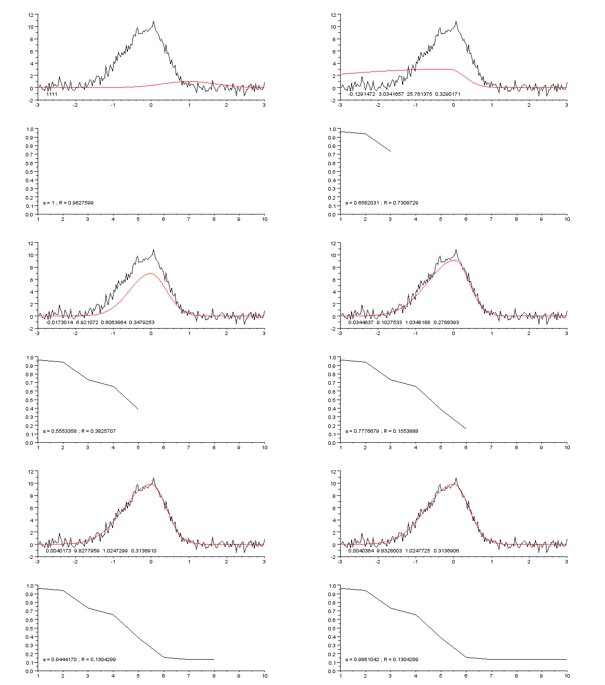
Interpolation versus approximation

A basic distinction is between interpolation and smoothing. Interpolation forces the fitted curve to pass through every data point and is useful when data are exact or when preserving known values is crucial. Approximation or smoothing yields a curve that captures the underlying trend while ignoring small-scale variability introduced by measurement error or noise. Related statistical frameworks, such as regression analysis, emphasize inference about uncertainty in fitted relationships and parameter estimates.

Common methods and models

Several families of models and algorithms are widely used:

• Linear least squares: fits linear combinations of basis functions (including straight lines and polynomials) by minimizing squared residuals.
• Polynomial fitting: represents the trend with a polynomial; higher degree increases flexibility but can cause oscillation and overfitting.
• Spline and piecewise models: use low-degree polynomials joined smoothly at knots to capture local behavior while controlling global shape.
• Nonlinear and parametric models: fit models where parameters enter nonlinearly; these require iterative optimization (for example, Gauss–Newton or Levenberg–Marquardt methods).
• Regularized and robust fits: add penalties or use alternative loss functions to limit overfitting and reduce sensitivity to outliers.

History and development

The mathematical foundations of curve fitting developed alongside statistics and numerical analysis. Early formalization of least squares methods dates to the work of mathematicians and astronomers in the early 19th century. Advances in spline theory, numerical linear algebra and computing power in the 20th century made complex, high-dimensional and nonparametric fits practical, broadening applications across science and engineering.

Applications and examples

Curve fitting appears across disciplines. In experimental sciences it summarizes measurements and supports interpolation between observations. Engineers use fitted curves for calibration and component characterization. Economists and social scientists use regression-based fits to explore relationships among variables. In machine learning, many supervised-learning methods can be viewed as sophisticated curve-fitting procedures that balance fit and generalization.

Practical considerations and pitfalls

When fitting curves it is important to diagnose model quality and to be cautious about extrapolation. Extrapolating beyond the observed range of the observed data can produce unreliable predictions because the fitted form may not reflect true behavior outside the data. Standard diagnostics include residual analysis, goodness-of-fit measures (for example, root-mean-square error and R-squared), cross-validation for selecting complexity or smoothing parameters, and inspection for heteroscedasticity or influential points. Weighting, robust loss functions, and regularization are practical tools to address measurement error and to prevent overfitting.

In routine practice, choosing a fitting strategy involves trade-offs between bias and variance, interpretability and flexibility, and sensitivity to noise. A careful combination of domain knowledge, diagnostic checks, and validation with independent data gives the most reliable outcomes when constructing curves from empirical observations.