
Brownian motion: random particle motion, theory and applications
Random jittery motion of small particles in fluids caused by molecular impacts; foundational to kinetic theory, diffusion, stochastic processes and applied models in science and finance.
Overview
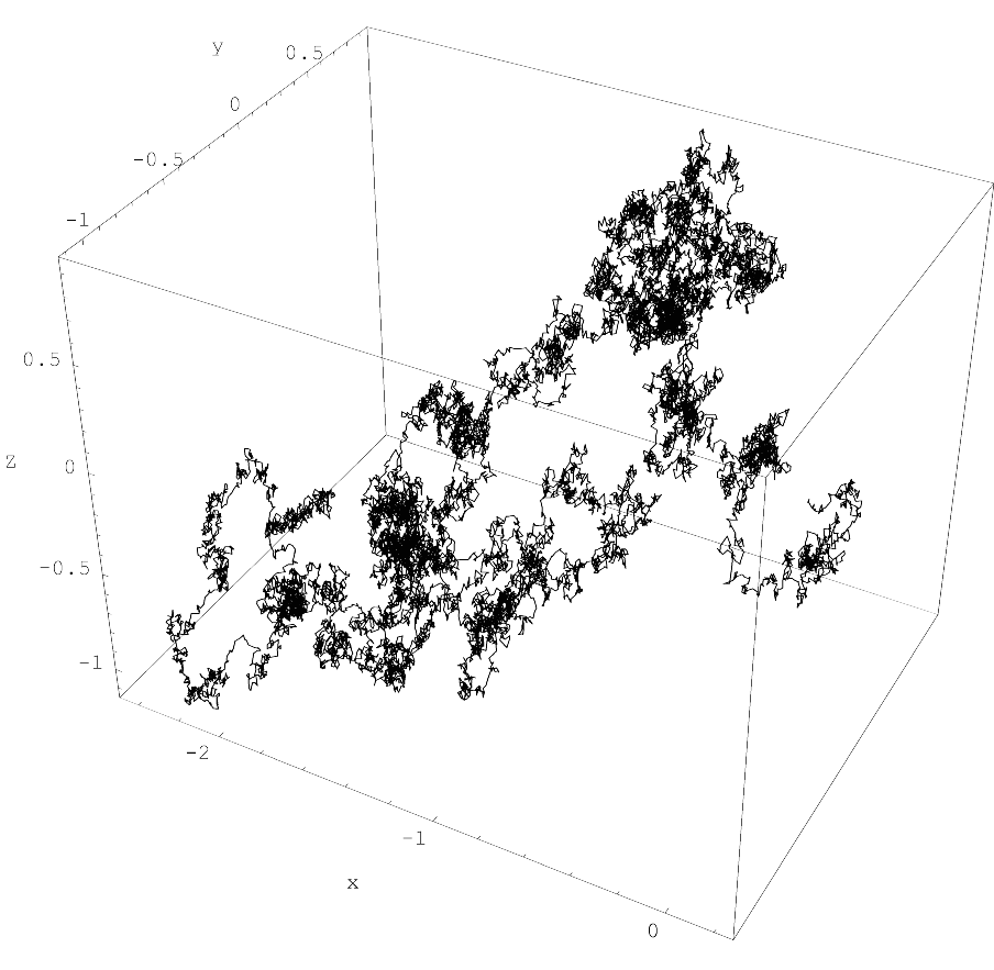
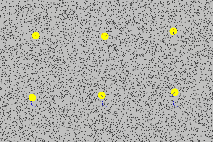
Brownian motion refers to the erratic, continuous movement observed for small particles suspended in a fluid. These suspended grains, droplets or colloidal particles exhibit an irregular trajectory when viewed under magnification. The motion arises because the particles are continually struck by much smaller and faster constituents of the medium: individual atoms and molecules. It is visible for solid specks in a liquid and for aerosol particles in a gas, and is a macroscopic manifestation of microscopic thermal activity.
Image gallery
7 Images



Historical background
The phenomenon was first described in 1827 by the botanist Robert Brown, who noticed the perpetual jiggling of tiny particles within pollen grains immersed in water. Brown observed the motion without identifying its cause. In the early 20th century, theoretical work by Albert Einstein and others connected these observations to the kinetic theory of matter: random molecular impacts produce the measurable wander of suspended particles. Experimental confirmation by Jean Perrin helped convince the scientific community of the reality of atoms and molecules, a contribution recognized by the Nobel Prize awarded to Perrin.
Physical mechanism and statistical description
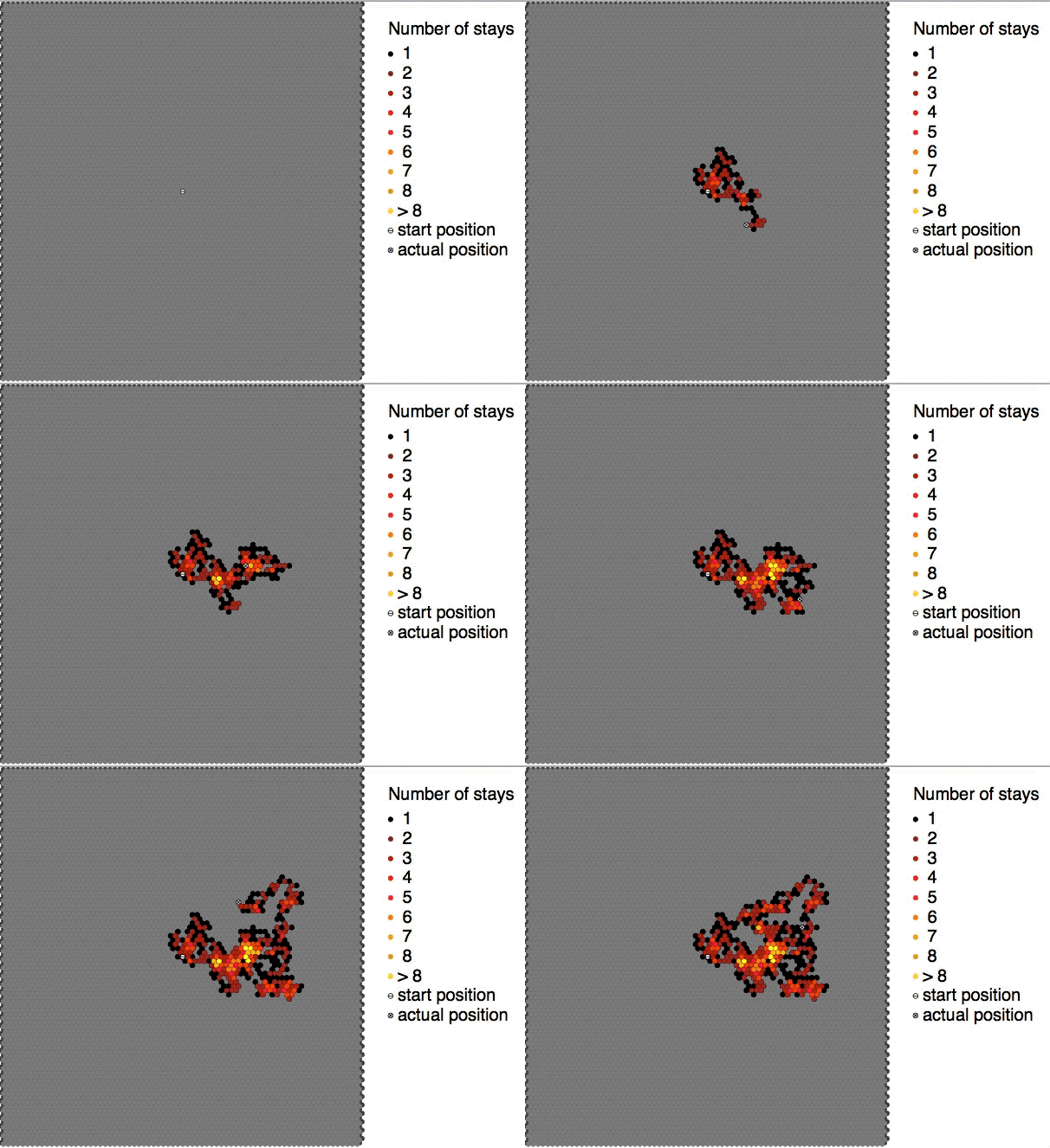
At thermal equilibrium the fluid's microscopic constituents constantly collide with a suspended particle. Because these impacts are numerous and random in direction and timing, the net force on the particle fluctuates in a way that produces an irregular path. Individual collisions cannot be tracked in practice, so the phenomenon is described statistically. Classical descriptions use ideas from statistical mechanics to connect microscopic motion with observable quantities like diffusion coefficients and mean squared displacement.
Mathematical models and properties
Mathematical treatments model the motion at different levels of idealization. A few common frameworks are:
- Langevin equation: a Newtonian balance with a random forcing term representing collisions.
- Fokker–Planck and diffusion equations: deterministic partial differential equations for probability densities.
- Stochastic process models: idealized random functions of time, notably the Wiener process, which capture essential probabilistic features.
In the simplest ideal, displacements over short time intervals are often modeled as independent, Gaussian random variables with zero mean and variance proportional to elapsed time. This scaling property — variance growing linearly with time — is a hallmark of classical diffusion and is related to limit theorems for random steps such as the random walk and stochastic process limits proved in results like Donsker's theorem. The continuous mathematical ideal of Brownian motion studied by Norbert Wiener is often called the Wiener process.
Applications and examples
Brownian motion is central to many areas of science and engineering. It provides the microscopic basis for diffusion and underlies Fick's laws used in chemistry and biology. Techniques that track Brownian motion help determine particle sizes and viscosities, calibrate microscopes, and measure thermal forces in soft-matter experiments. In physics, the Langevin and Fokker–Planck formalisms describe transport and relaxation. The same stochastic ideas have been adapted as models in quantitative finance (for example, geometric Brownian motion for asset prices), although such economic models are only analogies, not literal molecular phenomena.
Distinctions and notable facts
Important distinctions should be kept in mind: the physical phenomenon in a real fluid involves discrete collisions and hydrodynamic effects, whereas the Wiener process is an idealized continuous-time model with specific mathematical properties (continuous paths that are almost surely nowhere differentiable, Gaussian increments, and stationary independent increments). Various refinements address finite particle size, inertia, and correlated forces. For readers seeking further technical development and experimental methods, classic references mix statistical mechanics treatments with stochastic calculus and experimental reports; introductory paths often move from simple random walks to diffusion equations and finally to the Wiener process and its applications.
For concise introductions and historical notes, see sources on basic particle behavior and stochastic modeling: particles, liquid environments, gas environments, theoretical discussions of statistical mechanics and stochastic processes, classic treatments of the random walk, and mathematical expositions tied to Norbert Wiener. Historical figures connected to the discovery and explanation include Robert Brown, the early-20th-century theorists, and experimentalists honored with a Nobel Prize.
Questions and answers
Q: What is Brownian motion?
A: Brownian motion is the random motion of particles in a liquid or a gas caused by fast-moving atoms or molecules that hit the particles.
Q: Who discovered Brownian Motion?
A: Brownian Motion was discovered in 1827 by the botanist Robert Brown.
Q: How did Albert Einstein contribute to understanding Brownian Motion?
A: In 1905, Albert Einstein published a paper which explained how the motion observed by Robert Brown was caused by individual water molecules hitting the particles. This helped convince many scientists that atoms and molecules exist.
Q: Who verified Einstein's theory experimentally?
A: Jean Perrin verified Einstein's theory experimentally in 1908 and was awarded the Nobel Prize in Physics for his work on matter structure.
Q: How does this random pattern occur?
A: The direction of force from atomic bombardment constantly changes, leading to different sides of the particle being hit at different times and causing seemingly random patterns of movement.
Q: What kind of models are used to describe it? A: Probabilistic models of molecular populations such as those made by Einstein and Smoluchowski, as well as stochastic process models are used to describe it.
Q: Who else studied Brownian Movement with greater mathematical precision? A: Norbert Wiener also studied Brownian Movement with greater mathematical precision.
Related articles
Author
AlegsaOnline.com Brownian motion: random particle motion, theory and applications Leandro Alegsa
URL: https://en.alegsaonline.com/art/14799
Sources
- archive.org : Atoms