
Bose–Einstein statistics: occupancy rules and physical consequences
Bose–Einstein statistics describe how indistinguishable bosons occupy energy states, the distribution formula, historical origin, physical examples (photons, BECs) and limits compared with other statistics.
Overview
Bose–Einstein statistics is the rule set in statistical physics that governs how a collection of indistinguishable particles with integer spin — bosons — populate available quantum states. Unlike distinguishable particles or fermions, bosons can share the same quantum state in unlimited numbers, which leads to collective phenomena not present for particles that obey other statistics. For background on the general framework, see statistical mechanics.
Image gallery
2 Images
Distribution and basic formula
The average occupation number n(ε) of a single-particle state with energy ε at thermal equilibrium and temperature T is given by the Bose–Einstein distribution. In compact form it reads n(ε) = 1/(exp((ε − μ)/kT) − 1), where μ is the chemical potential and k is Boltzmann's constant. This formula applies for energies above the chemical potential (ε > μ) and shows the tendency of bosons to accumulate into low-energy states.
Key characteristics
Important features of Bose–Einstein statistics include:
- Indistinguishability: Particles are counted without labels; see indistinguishability and its consequences for entropy and counting.
- Bosonic nature: The particles obey Bose–Einstein rules because they are bosons; canonical examples are the boson family and the photon.
- Unlimited occupancy: Any number of particles can occupy the same single-particle state, which permits macroscopic occupation numbers at low energy.
Historical development
The distribution is named after Satyendra Nath Bose and Albert Einstein. Bose developed a derivation of photon statistics that treated quanta as indistinguishable, and Einstein extended the approach to massive particles, predicting the possibility of a phase transition where particles condense into the ground state at low temperature. The theory links microscopic state counting to macroscopic thermodynamic behavior of a quantum system.
Examples and physical importance
Bose–Einstein statistics underlie many familiar phenomena: the distribution of photons in blackbody radiation, the operation of lasers, superfluidity in liquid helium, and the formation of Bose–Einstein condensates (BECs) in dilute atomic gases. In applications one tracks how the occupation n(ε) varies with energy, the chemical potential, and the temperature to predict measurable properties such as specific heat, coherence, and condensate fraction. Experimental systems range from light in optical cavities to cold atoms trapped in magnetic or optical potentials.
Distinctions, limits and approximations
Bose–Einstein statistics differ from Fermi–Dirac statistics (for half-integer spin particles) by allowing multiple occupancy, and from classical Maxwell–Boltzmann statistics by quantum indistinguishability. In the high-energy or high-temperature limit, when (ε − μ) ≫ kT, the Bose–Einstein formula reduces to the classical Maxwell–Boltzmann form and quantum effects become negligible. When conditions allow very large occupation of the lowest state, one observes Bose–Einstein condensation, a macroscopic quantum state with distinct thermodynamic signatures.
Further reading
For more details and mathematical derivations, follow topics on the Bose–Einstein distribution, comparisons with Maxwell–Boltzmann behavior, and resources describing experimental realizations and implications for condensed matter and optical physics.

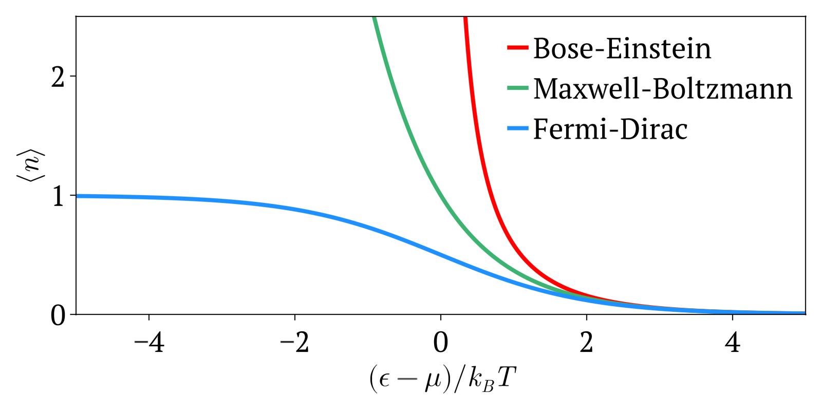
Occupation number ⟨  as a function of the energy
for bosons (Bose-Einstein statistics, upper curve)
or fermions (Fermi-Dirac statistics, lower curve),
in each case in the special case of interaction freedom and at constant temperature
The chemical potential μ  is a parameter that depends on temperature and density;
in the Bose case it is always smaller than the energy and would vanish in the limiting case of Bose-Einstein condensation;
in the Fermi case, however, it is positive, at  it corresponds to the Fermi energy.
With freedom from interaction
If there is no interaction (bosegas), the following formula results for bosons:
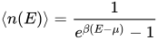
with
- the chemical potential μ
 which for bosons is always smaller than the lowest possible energy value: μ therefore
the Bose-Einstein statistics is
only for energy values E - μ - of the energy normalization β
 . The choice of β temperature scale used:
 - usually it is chosen to be β
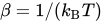 with Boltzmann constant
  ;
; - it is β
 when the temperature is measured in energy units, such as joules; this occurs when also does not appear in the definition of entropy-which is then unitless.
Below a very low critical temperature  one obtains Bose-Einstein condensation under interaction freedom - assuming that μ
  tends towards the energy minimum.
Note that ⟨  the occupation number of a quantum state. If one needs the occupation number of a degenerate energy level, the above expression has to be multiplied additionally by the corresponding degeneracy
  (
(  : spin, for bosons always integer), cf. also multiplicity.
Related articles
Author
AlegsaOnline.com Bose–Einstein statistics: occupancy rules and physical consequences Leandro Alegsa
URL: https://en.alegsaonline.com/art/13182