Binomial distribution

The binomial distribution is one of the most important discrete probability distributions.

It describes the number of successes in a series of similar and independent experiments, each of which has exactly two possible outcomes ("success" or "failure"). Such series of experiments are also called Bernoulli processes.

If the probability of success on an attempt and the number of attempts, then denote by $B(k\mid p,n)$ (also $B_{n,p}(k)$ , B(n,p,k) or B(n;p;k) ) is the probability of achieving exactly successes (see section Definition).

The binomial distribution and the Bernoulli test can be illustrated with the help of the Galton board. This is a mechanical apparatus into which balls are thrown. These then fall randomly into one of several compartments, where the distribution corresponds to the binomial distribution. Depending on the construction, different parameters and are possible.

Although the binomial distribution was known long before, the term was first used in 1911 in a book by George Udny Yule.

Probability function of binomial distribution for n=20 ; p=0{,}1 (blue), p=0{,}5 (green) and p=0{,}8 (red)

Binomial distributions for p=0{,}5
with and as in Pascal's triangle.

The probability that a ball in a Galton board with eight levels ( n=8 ) falls into the middle compartment ( k=4 ) is 70/256 .

Examples

The probability of rolling a number greater than 2 with a normal die is $p={\tfrac {4}{6}}={\tfrac {2}{3}}$ ; the probability that this is not the case is $q=1-p={\tfrac {1}{3}}$ . Suppose one rolls the dice 10 times ( n=10 ) , then there is a small probability that no number greater than 2 is rolled a single time, or conversely every time. The probability of rolling -times rolling such a number $(0\leq k\leq 10)$ , is $B_{n,p}(k)$ described by the binomial distribution

The process described by the binomial distribution is often illustrated by a so-called urn model. In an urn, for example, there are 6 balls, 2 of them black, the others white. Reach into the urn 10 times, take out one ball, note its color and put the ball back. In a special interpretation of this process, drawing a white ball is understood as a "positive event" with probability , drawing a non-white ball as a "negative result". The probabilities are distributed in the same way as in the previous example of rolling the dice.

Definition

Probability function, (cumulative) distribution function, properties

The discrete probability distribution with the probability function

$B(k\mid p,n)={\begin{cases}{\binom {n}{k}}p^{k}(1-p)^{n-k}&{\text{falls}}\quad k\in \left\{0,1,\dots ,n\right\}\\0&{\text{sonst.}}\end{cases}}$

is called the binomial distribution for the parameters (number of trials) and $p\in \left[0,1\right]$ (the success or hit probability).

Note: This formula uses the convention 0^0:=1 (see zero to the power of zero).

The above formula can be understood like this: We need for a total of trials exactly successes of probability $p^{k}$ and consequently have exactly n-k failures of probability $(1-p)^{n-k}$ . However, each of the successes occur on each of the trials, so we still have to deal with the number ${\tbinom {n}{k}}$ of -elementary subsets of an -elementary set. This is because there are exactly as many ways to select the successful ones from all trials.

The failure probability 1-p complementary to the success probability is often abbreviated as

As necessary for a probability distribution, the probabilities for all possible values must sum to 1. This follows from the binomial theorem as follows:

$\sum _{k=0}^{n}{\binom {n}{k}}p^{k}(1-p)^{n-k}=\left(p+\left(1-p\right)\right)^{n}=1^{n}=1$

A random variable $B(\cdot \mid p,n)$ distributed according to is accordingly calledbinomially distributed with parameters and and distribution function

$F_{X}(x)=\operatorname {P} (X\leq x)=\sum _{k=0}^{\lfloor x\rfloor }{\binom {n}{k}}p^{k}(1-p)^{n-k}$ ,

where ⌊ $\lfloor x\rfloor$ denotes the rounding function.

Other common notations of the cumulative binomial distribution are $F(k\mid p,n)$ , F(n,p,k) and F(n;p;k) .

Derivation as Laplace probability

Experiment scheme: An urn contains balls, of which are black and N-M white. The probability of drawing a black ball is therefore $p={\frac {M}{N}}$ . One by one, balls are taken at random, their color is determined, and they are put back.

We calculate the number of possibilities in which black balls can be found, and from this we calculate the so-called Laplace probability ("number of possibilities favorable to the event divided by the total number of (equally probable) possibilities").

For each of the draws, there are possibilities, so in total there are $N^{n}$ possibilities for the choice of balls. For exactly of these balls to be black, exactly of the draws must have a black ball. For each black ball, there are possibilities, and for each white ball N-M possibilities. The black balls may still be distributed in ${\tbinom {n}{k}}$ possible ways over the draws, so there are

${\binom {n}{k}}M^{k}(N-M)^{n-k}$

Cases where exactly black balls have been selected. The probability of $p_{k}$ finding exactly } black balls among is thus:

${\begin{aligned}p_{k}&={\binom {n}{k}}{\frac {M^{k}(N-M)^{n-k}}{N^{n}}}\\&={\binom {n}{k}}\left({\frac {M}{N}}\right)^{k}\left({\frac {N-M}{N}}\right)^{n-k}\\&={\binom {n}{k}}p^{k}(1-p)^{n-k}\end{aligned}}$

Properties

Symmetry

The binomial distribution is symmetric in the special cases , and symmetric and otherwise asymmetric.
The binomial distribution has the property

Expected value

The binomial distribution has the expected value .

Proof

The expected value μ $\mu$ calculated directly from the definition μ $\mu =\sum _{i=1}^{n}x_{i}p_{i}$ and the binomial theorem of

${\begin{aligned}\mu &=\sum _{k=0}^{n}k{\binom {n}{k}}p^{k}(1-p)^{n-k}\\&=np\sum _{k=0}^{n}k{\frac {(n-1)!}{(n-k)!k!}}p^{k-1}(1-p)^{(n-1)-(k-1)}\\&=np\sum _{k=1}^{n}{\frac {(n-1)!}{(n-k)!(k-1)!}}p^{k-1}(1-p)^{(n-1)-(k-1)}\\&=np\sum _{k=1}^{n}{\binom {n-1}{k-1}}p^{k-1}(1-p)^{(n-1)-(k-1)}\\&=np\sum _{\ell =0}^{n-1}{\binom {n-1}{\ell }}p^{\ell }(1-p)^{(n-1)-\ell }\quad {\text{mit }}\ell :=k-1\\&=np\sum _{\ell =0}^{m}{\binom {m}{\ell }}p^{\ell }(1-p)^{m-\ell }\qquad {\text{mit }}m:=n-1\\&=np\left(p+\left(1-p\right)\right)^{m}=np1^{m}=np.\end{aligned}}$

Alternatively, use that a $B(\cdot \mid p,n)$ -distributed random variable as a sum of independent Bernoulli distributed random variables $X_{i}$ with $\operatorname {E} (X_{i})=p$ can be written. With the linearity of the expected value then follows

$\operatorname {E} (X)=\operatorname {E} (X_{1}+\dotsb +X_{n})=\operatorname {E} (X_{1})+\dotsb +\operatorname {E} (X_{n})=np.$

Alternatively, one can also give the following proof using the binomial theorem: If one differentiates at the equation

$(a+b)^{n}=\sum _{k=0}^{n}{\tbinom {n}{k}}a^{k}b^{n-k}$

both sides to , results in

$n(a+b)^{n-1}=\sum _{k=0}^{n}k{\tbinom {n}{k}}a^{k-1}b^{n-k}$ ,

$na(a+b)^{n-1}=\sum _{k=0}^{n}k{\tbinom {n}{k}}a^{k}b^{n-k}$ .

With a=p and the desired result follows. b=1-p

Variance

The binomial distribution has variance npq with q=1-p .

Proof

be a B(n,p) -distributed random variable. The variance is determined directly from the shift theorem $\operatorname {Var} (X)=\operatorname {E} \left(X^{2}\right)-\left(\operatorname {E} \left(X\right)\right)^{2}$ to

$\operatorname {Var} (X)=\sum _{k=0}^{n}k^{2}\cdot P(X=k)-(np)^{2}$

$=\sum _{k=0}^{n}k^{2}\cdot {n \choose k}p^{k}(1-p)^{n-k}-n^{2}p^{2}$

$={\cancel {n^{2}p^{2}}}-np^{2}+np{\cancel {-n^{2}p^{2}}}$

$=np(1-p)=npq$

or, alternatively, from Bienaymé's equation applied to the variance of independent random variables, considering that the identical individual processes $X_{i}$ $\operatorname {Var} (X_{i})=p(1-p)=pq$ satisfy the Bernoulli distribution with becomes

$\operatorname {Var} (X)=\operatorname {Var} (X_{1}+\dotsb +X_{n})=\operatorname {Var} (X_{1})+\dotsb +\operatorname {Var} (X_{n})=n\operatorname {Var} (X_{1})=np\left(1-p\right)=npq.$

The second equality holds because the individual experiments are independent, so the individual variables are uncorrelated.

Coefficient of variation

From the expected value and variance one obtains the coefficient of variation

$\operatorname {VarK} (X)={\sqrt {\frac {1-p}{np}}}.$

Skew

The skewness results to

$\operatorname {v} (X)={\frac {1-2p}{\sqrt {np(1-p)}}}.$

Camber

The curvature can also be represented closed as

$\beta _{2}=3+{\frac {1-6pq}{npq}}.$

Thus the excess

$\gamma ={\frac {1-6pq}{npq}}.$

Mode

The mode, i.e. the value with the maximum probability, is for p<1 k = ⌊ $k=\lfloor np+p\rfloor$ for p = 1 {\displaystyle p=1 n {\displaystyle If np+p a natural number, k=np+p-1 also a mode. If the expected value is a natural number, the expected value is equal to the mode.

Proof

Let be without restriction We consider the quotient

$\alpha _{k}:={\frac {B(k+1\mid p,n)}{B(k\mid p,n)}}={\frac {\,{\frac {n!}{(k+1)!(n-k-1)!}}\,}{\frac {n!}{k!(n-k)!}}}\cdot {\frac {p^{k+1}(1-p)^{n-k-1}}{p^{k}(1-p)^{n-k}}}={\frac {n-k}{k+1}}\cdot {\frac {p}{1-p}}$ .

Now α $\alpha _{k}>1$ , if k<np+p-1 k < $\alpha _{k}<1$ , if Thus:

${\begin{aligned}k>(n+1)p-1\Rightarrow \alpha _{k}<1\Rightarrow B(k+1\mid p,n)<B(k\mid p,n)\\k=(n+1)p-1\Rightarrow \alpha _{k}=1\Rightarrow B(k+1\mid p,n)=B(k\mid p,n)\\k<(n+1)p-1\Rightarrow \alpha _{k}>1\Rightarrow B(k+1\mid p,n)>B(k\mid p,n)\end{aligned}}$

And only in the case the quotient $np+p-1\in \mathbb {N}$ has the value 1, i.e. $B(np+p-1\mid n,p)=B(np+p\mid n,p)$ .

Median

It is not possible to give a general formula for the median of the binomial distribution. Therefore, different cases have to be considered which provide a suitable median:

If is a natural number, then the expected value, median, and mode agree and are equal to .
A median lies in the interval ⌊ $\lfloor np\rfloor \leq m\leq \lceil np\rceil$ . Here, ⌊ denote $\lfloor \cdot \rfloor$ the rounding function and ⌈ $\lceil \cdot \rceil$ denote the rounding up function.
A median cannot deviate too much from the expected value: $|m-np|\leq \min\{\ln 2,\max\{p,1-p\}\}$ .
The median is unique and coincides with $m=$ round $(np)$ if either $p\leq 1-\ln 2$ or $p\geq \ln 2$ or $|m-np|\leq \min\{p,1-p\}$ (except when and is even).
If and is odd, then every number in the interval $1/2(n-1)\leq m\leq 1/2(n+1)$ a median of the binomial distribution with parameters and . If and is even, then $m=n/2$ the unique median.

Cumulants

Analogous to the Bernoulli distribution, the cumulant generating function is

$g_{X}(t)=n\ln(pe^{t}+q)$ .

Thus, the first cumulants κ $\kappa _{1}=np,\kappa _{2}=npq$ and the recursion equation holds.

$\kappa _{k+1}=p(1-p){\frac {d\kappa _{k}}{dp}}.$

Characteristic function

The characteristic function has the form

$\phi _{X}(s)=\left(\left(1-p\right)+p\mathrm {e} ^{\mathrm {i} s}\right)^{n}=\left(q+p\mathrm {e} ^{\mathrm {i} s}\right)^{n}.$

Probability generating function

For the probability generating function we get

$g_{X}(s)=(ps+(1-p))^{n}.$

Moment generating function

The moment generating function of the binomial distribution is

${\begin{aligned}m_{X}(s)&=\operatorname {E} \left(e^{sX}\right)\\&=\sum _{k=0}^{n}\mathrm {e} ^{sk}\cdot {\binom {n}{k}}p^{k}(1-p)^{n-k}\\&=\sum _{k=0}^{n}{\binom {n}{k}}(\mathrm {e} ^{s}p)^{k}(1-p)^{n-k}\\&=\left(p\cdot \mathrm {e} ^{s}+\left(1-p\right)\right)^{n}.\end{aligned}}$

Sum of binomial distributed random variables

For the sum Z=X+Y two independent binomial distributed random variables and with parameters $n_{1}$ , and $n_{2}$ , the individual probabilities are obtained by applying Vandermonde's identity

${\begin{aligned}\operatorname {P} (Z=k)&=\sum _{i=0}^{k}\left[{\binom {n_{1}}{i}}p^{i}(1-p)^{n_{1}-i}\right]\left[{\binom {n_{2}}{k-i}}p^{k-i}(1-p)^{n_{2}-k+i}\right]\\&={\binom {n_{1}+n_{2}}{k}}p^{k}(1-p)^{n_{1}+n_{2}-k}\qquad (k=0,1,\dotsc ,n_{1}+n_{2}),\end{aligned}}$

thus again a binomially distributed random variable, but with the parameters $n_{1}+n_{2}$ and . Thus for the convolution

$\operatorname {Bin} (n,p)*\operatorname {Bin} (m,p)=\operatorname {Bin} (n+m,p)$

Thus, the binomial distribution is reproductive for fixed or forms a convolution semigroup.

If the sum Z=X+Y is known, each of the random variables and follows a hypergeometric distribution under this condition. To do this, one calculates the conditional probability:

${\begin{aligned}P(X=\ell |Z=k)&={\frac {P(X=\ell \cap Z=k)}{P(Z=k)}}\\&={\frac {P(X=\ell \cap Y=k-\ell )}{P(Z=k)}}\\&={\frac {P(X=\ell )P(Y=k-\ell )}{P(Z=k)}}\\&={\frac {{\binom {n_{1}}{\ell }}p^{\ell }(1-p)^{n_{1}-\ell }{\binom {n_{2}}{k-\ell }}p^{k-\ell }(1-p)^{n_{2}-k+\ell }}{{\binom {n_{1}+n_{2}}{k}}p^{k}(1-p)^{n_{1}+n_{2}-k}}}\\&={\frac {{\binom {n_{1}}{\ell }}{\binom {n_{2}}{k-\ell }}}{\binom {n_{1}+n_{2}}{k}}}\\&=h(\ell ;n_{1}+n_{2};n_{1};k)\end{aligned}}$

This represents a hypergeometric distribution.

In general: If the random variables $X_{i}$ are stochastically independent and $B(n_{i},p)$ satisfy the binomial distributions then the sum $X_{1}+X_{2}+\dotsb +X_{m}$ is also binomially distributed, but with parameters $n_{1}+n_{2}+\dotsb +n_{m}$ and . Adding binomially distributed random variables $X_{1},X_{2}$ with $p_{1}\neq p_{2}$ , then a generalized binomial distribution is obtained.

Relationship to other distributions

Relationship to Bernoulli distribution

A special case of the binomial distribution for n=1 is the Bernoulli distribution. The sum of independent and identical Bernoulli distributed random variables therefore satisfies the binomial distribution.

Relationship to the generalized binomial distribution

The binomial distribution is a special case of the generalized binomial distribution with $p_{i}=p_{j}$ for all $i,j\in \{1,\dotsc ,n\}$ . More precisely, for fixed expected value and fixed order, it is the one generalized binomial distribution with maximum entropy.

Transition to normal distribution

According to Moivre-Laplace's theorem, the binomial distribution converges to a normal distribution in the limiting case $n\to \infty$ , i.e., the normal distribution can be used as a useful approximation of the binomial distribution if the sample size is sufficiently large and the proportion of the expression sought is not too small. The Galton board can be used to experimentally recreate the approximation to the normal distribution.

It holds μ $\mu =np$ and σ $\sigma ^{2}=npq.$ Substituting in the distribution function $\Phi$ of the standard normal distribution, it follows.

$B(k\mid p,n)\approx \Phi \left({k+0{,}5-np \over {\sqrt {npq}}}\right)-\ \Phi \left({k-0{,}5-np \over {\sqrt {npq}}}\right)\approx {1 \over {\sqrt {npq}}}\cdot \ {\frac {1}{\sqrt {2\pi }}}\,\cdot \ \exp \left(-{{(k-np)}^{2} \over 2npq}\right).$

As can be seen, the result is thus nothing but the function value of the normal distribution for $x=k$ , μ $\mu =n\cdot p$ as well as σ $\sigma ^{2}=n\cdot p\cdot q$ (which can be visualized also as the area of the -th strip of the histogram of the standardized binomial distribution with $1/\sigma$ as its width and $\Phi ((k-\mu )/\sigma )$ as its height). The approximation of the binomial distribution to the normal distribution is used in the normal approximation to quickly determine the probability of many levels of the binomial distribution, especially when no (more) table values are available for them.

Transition to Poisson distribution

An asymptotically asymmetric binomial distribution whose expected value for $n\rightarrow \infty$ and $p\rightarrow 0$ $\lambda$ converges to a constant λ can be approximated by the Poisson distribution. The value λ $\lambda$ is then the expected value for all the binomial distributions considered in the limit calculation as well as for the resulting Poisson distribution. This approximation is also called Poisson approximation, Poisson limit theorem or the law of rare events.

${\begin{aligned}B(k\mid p,n)&={n \choose k}p^{k}\,(1-p)^{n-k}={\frac {n!}{(n-k)!\,k!}}\left({\frac {np}{n}}\right)^{k}\left(1-{\frac {np}{n}}\right)^{n-k}\\&={\frac {n(n-1)(n-2)\dotsm (n-k+1)}{n^{k}}}\,{\frac {(np)^{k}}{k!}}\left(1-{\frac {np}{n}}\right)^{n-k}\\&=\left(1-{\frac {1}{n}}\right)\left(1-{\frac {2}{n}}\right)\dotsm \left(1-{\frac {k-1}{n}}\right){\frac {(np)^{k}}{k!}}\left(1-{\frac {(np)}{n}}\right)^{n-k}\\&\to \,{\frac {\lambda ^{k}}{k!}}\mathrm {e} ^{-\lambda },\quad {\text{wenn}}\quad n\to \infty \quad {\text{und}}\quad p\rightarrow 0\end{aligned}}$

A rule of thumb is that this approximation is useful when $n\geq 50$ and $p\leq 0{,}05$ .

The Poisson distribution is therefore the limiting distribution of the binomial distribution for large and small , it is convergence in distribution.

Relationship to geometric distribution

The number of failures until a success occurs for the first time is described by the geometric distribution.

Relationship to the negative binomial distribution

The negative binomial distribution, on the other hand, describes the probability distribution of the number of trials required to achieve a given number of successes in a Bernoulli process.

Relationship to hypergeometric distribution

In the binomial distribution, the selected samples are returned to the selected set, so they can be selected again at a later time. In contrast, if the samples are not returned to the population, the hypergeometric distribution is used. The two distributions merge when the size the population is large and the size the samples is small. As a rule of thumb, for $n/N\leq 0{,}05$ the binomial distribution can be used instead of the mathematically more demanding hypergeometric distribution even if the samples are not taken, since in this case both yield only insignificantly different results.

Relationship to multinomial distribution

The binomial distribution is a special case of the multinomial distribution.

Relationship to Rademacher distribution

If binomially distributed for parameter p=0{,}5 and , then $X_1, \dotsc, X_n$ represented as a scaled sum of Rademacher distributed random variables

$Y=0{,}5\left(n+\sum _{i=1}^{n}X_{i}\right)$

This is used in particular for the symmetric random walk on $\mathbb {Z}$ used.

Relationship to Panjer distribution

The binomial distribution is a special case of the Panjer distribution, which combines the distributions binomial distribution, negative binomial distribution and Poisson distribution in one distribution class.

Relationship to beta distribution

For many applications it is necessary to use the distribution function

$\sum _{i=0}^{k}B(i\mid p,n)$

concretely (for example, for statistical tests or for confidence intervals).

The following relationship to beta distribution helps here:

$\sum _{i=0}^{k}{\binom {n}{i}}\cdot p^{i}\cdot (1-p)^{n-i}=\operatorname {Beta} (1-p;n-k;k+1)$

This is for integer positive parameters and :

$\operatorname {Beta} (x;a;b)={(a+b-1)! \over (a-1)!\cdot (b-1)!}\int _{0}^{x}u^{a-1}(1-u)^{b-1}\,\mathrm {d} u$

To solve the equation

$\sum _{i=0}^{k}{\binom {n}{i}}\cdot p^{i}\cdot (1-p)^{n-i}={n! \over (n-k-1)!\cdot k!}\int _{0}^{1-p}u^{n-k-1}(1-u)^{k}\,\mathrm {d} u$

to prove, you can proceed as follows:

The left and right sides match for (both sides are equal to 1).
The derivatives with respect to left and right sides of the equation, namely they are both equal $-{n! \over (n-k-1)!\cdot k!}\cdot p^{k}\cdot (1-p)^{n-k-1}$ .

Relationship to beta binomial distribution

A binomial distribution whose parameter beta distributed is called a beta binomial distribution. It is a mixture distribution.

Relationship to the Pólya distribution

The binomial distribution is a special case of the Pólya distribution (choose c=0 ).

Examples

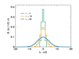
Symmetric binomial distribution (p = 1/2)

p = 0.5 and n = 4, 16, 64

Mean value subtracted

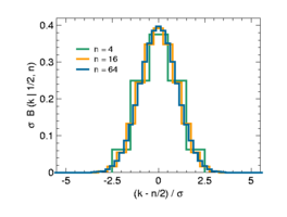
Scaling with standard deviation

This case occurs for the -fold coin toss with a fair coin (probability for heads equal to that for tails, so equal to 1/2). The first figure shows the binomial distribution for p=0{,}5 and for different values of as a function of . These binomial distributions are mirror symmetric about the value k=n/2 :

$B(k\mid 1/2;n)=B(n-k\mid 1/2;n)$

This is illustrated in the second figure. The width of the distribution grows in proportion to the standard deviation σ $\sigma ={\frac {\sqrt {n}}{2}}$ . The function value at k=n/2 , i.e. the maximum of the curve, decreases proportionally to σ $\sigma$ .

Accordingly, binomial distributions with different can be scaled to each other by $\sigma$ dividing the abscissa k-n/2 by σ and $\sigma$ multiplying the ordinate by σ (third figure above).

The adjacent graph shows rescaled binomial distributions again, now for other values of and in a plot that better illustrates that all function values converge to a common curve with increasing By applying the Stirling formula to the binomial coefficients, we see that this curve (solid black in the figure) is a Gaussian bell curve:

$f(x)={\frac {1}{\sqrt {2\pi }}}\,{\mathrm {e} }^{-{\frac {x^{2}}{2}}}$ .

This is the probability density to the standard normal distribution ${\mathcal {N}}(0,1)$ . In the central limit theorem, this finding is generalized so that sequences of other discrete probability distributions also converge to the normal distribution.

The second graph on the right shows the same data in a semi-logarithmic plot. This is recommended if you want to check whether rare events that deviate from the expected value by several standard deviations also follow a binomial or normal distribution.

Pulling balls

There are 80 balls in a container, 16 of which are yellow. A ball is removed 5 times and then put back again. Because of the putting back, the probability of drawing a yellow ball is the same for all removals, namely 16/80 = 1/5. The value $B\left(k\mid {\tfrac {1}{5}};5\right)$ gives the probability that exactly the removed balls are yellow. As an example, we calculate k=3 :

$B\left(3\mid {\tfrac {1}{5}};5\right)={\binom {5}{3}}\cdot \left({\frac {1}{5}}\right)^{3}\cdot \left({\frac {4}{5}}\right)^{2}={\frac {5\cdot 4}{1\cdot 2}}\cdot {\frac {1}{125}}\cdot {\frac {16}{25}}={\frac {64}{1250}}=0{,}0512$

So in about 5% of the cases you draw exactly 3 yellow balls.

B(k \| 0.2; 5)
k	Probability in %
0	0032,768
1	0040,96
2	0020,48
3	0005,12
4	0000,64
5	0000,032
∑	0100
Erw.value	0001
Variance	0000.8

Number of people with birthday at the weekend

The probability that a person has a birthday on a weekend this year is (for simplicity) 2/7. There are 10 people in a room. The value $B(k\mid 2/7;10)$ indicates (in the simplified model) the probability that exactly of the people present have a birthday on a weekend this year.

B(k \| 2/7; 10)
k	Probability in % (rounded)
0	0003,46
1	0013,83
2	0024,89
3	0026,55
4	0018,59
5	0008,92
6	0002,97
7	0000,6797
8	0000,1020
9	0000,009063
10	0000,0003625
∑	0100
Erw.value	0002,86
Variance	0002,04

Common birthday in the year

253 people have come together. The value $B(k\mid 1/365;253)$ indicates the probability that exactly present have a birthday on a randomly chosen day (ignoring the year).

B(k \| 1/365; 253)
k	Probability in % (rounded)
0	049,95
1	034,72
2	012,02
3	002,76
4	000,47

Thus, the probability that "anyone" of these 253 people, i.e., one or more people, has a birthday on that day is $1-B(0\mid 1/365;253)=50.05\,\%$ .

For 252 persons, the probability is $1-B(0\mid 1/365;252)=49.91\,\%$ . That is, the threshold of the number of individuals above which the probability that at least one of these individuals has a birthday on a randomly chosen day becomes greater than 50% is 253 individuals (see also Birthday Paradox).

The direct calculation of the binomial distribution can be difficult due to the large factorials. An approximation via the Poisson distribution is permissible here ( With the parameter λ $\lambda =np=253/365$ following values result:

P253/365(k)
k	Probability in % (rounded)
0	050
1	034,66
2	012,01
3	002,78
4	000,48

Confidence interval for a probability

In an opinion poll among persons, individuals indicate that they will vote for party A. Determine a 95% confidence interval for the unknown proportion of voters who vote for party A in the total electorate.

A solution to the problem without recourse to the normal distribution can be found in the article Confidence Interval for the Success Probability of the Binomial Distribution.

Utilization model

The following formula can be used to calculate the probability that of people perform an activity that takes an average of minutes per hour simultaneously.

$P(X=k)={n \choose k}\cdot \left({\frac {m}{60}}\right)^{k}\cdot \left(1-{\frac {m}{60}}\right)^{n-k}$

Statistical error of class frequency in histograms

The display of independent measurement results in a histogram leads to the grouping of the measured values into classes.

The probability for $n_{i}$ entries in class is given by the binomial distribution

$B_{n,p_{i}}(n_{i})$ with $n=\sum n_{i}$ and $p_{i}={\frac {n_{i}}{n}}$ .

Expected value and variance of $n_{i}$ are then

$E(n_{i})=np_{i}=n_{i}$ and $V(n_{i})=np_{i}(1-p_{i})=n_{i}\left(1-{\frac {n_{i}}{n}}\right)$ .

Thus, the statistical error of the number of entries in class is

$\sigma (n_{i})={\sqrt {n_{i}\left(1-{\frac {n_{i}}{n}}\right)}}$ .

When the number of classes is large, becomes $p_{i}$ small and σ $\sigma (n_{i})\approx {\sqrt {n_{i}}}$ .

For example, the statistical accuracy of Monte Carlo simulations can be determined.

The same data in semi-logarithmic order

Binomial distributions with p = 0.5 (with shift by -n/2 and scaling) for n = 4, 6, 8, 12, 16, 23, 32, 46

Random numbers

Random numbers for the binomial distribution are usually generated using the inversion method.

Alternatively, one can exploit the fact that the sum of Bernoulli distributed random variables is binomially distributed. To do this, one generates Bernoulli distributed random numbers and sums them up; the result is a binomially distributed random number.

Binomial distribution

Examples

Definition

Probability function, (cumulative) distribution function, properties

Derivation as Laplace probability

Properties

Symmetry

Expected value

Variance

Coefficient of variation

Skew

Camber

Mode

Median

Cumulants

Characteristic function

Probability generating function

Moment generating function

Sum of binomial distributed random variables

Relationship to other distributions

Relationship to Bernoulli distribution

Relationship to the generalized binomial distribution

Transition to normal distribution

Transition to Poisson distribution

Relationship to geometric distribution

Relationship to the negative binomial distribution

Relationship to hypergeometric distribution

Relationship to multinomial distribution

Relationship to Rademacher distribution

Relationship to Panjer distribution

Relationship to beta distribution

Relationship to beta binomial distribution

Relationship to the Pólya distribution

Examples

Symmetric binomial distribution (p = 1/2)

Pulling balls

Number of people with birthday at the weekend

Common birthday in the year

Confidence interval for a probability

Utilization model

Statistical error of class frequency in histograms

Random numbers

Search by letter