Vector space

A vector space is a set of objects called vectors closed under addition and scalar multiplication; it is the central structure of linear algebra with bases, dimension and many applications.

Author: Leandro Alegsa Created: November 13, 2022 Updated: April 23, 2026

A vector space is a mathematical structure that abstracts the familiar properties of geometric vectors and extends them to many other kinds of objects. In everyday language a vector is any element of the space; see vectors for the general notion. A vector space equips that collection with two compatible procedures: a rule for combining two vectors (often called operations) and a rule for scaling a vector by a number. The first is typically referred to as addition and the second as scalar multiplication. Scalars themselves belong to a numerical system called a field; the elements used in scaling are called scalars.

$U$

Image gallery

2 Images

simple.wikipedia.org · Public domain

Formal definition and core properties

Formally, a vector space over a field F is a set V together with two operations that satisfy a fixed list of axioms: closure, associativity and commutativity of addition, existence of an additive identity and additive inverses, distributive laws connecting addition and scalar multiplication, and compatibility of scalar multiplication with multiplication in the field. This description links basic ideas from group theory (the additive structure) with properties of a field of scalars. The subject built on these axioms is linear algebra, which studies linear combinations, linear maps and systems that preserve the vector space structure.

Geometric vectors drawn as arrows provide an intuition: add two arrows by placing the tail of one at the head of the other; scale an arrow by stretching or shrinking it. However, the notion of vector is far more general: functions, sequences, polynomials and matrices are common examples when viewed as elements of a vector space. See examples such as spaces of functions and matrices for practical instances.

Representations and examples

Euclidean space R^n: familiar n-tuples of numbers with componentwise addition and real scalar multiplication.
Polynomial spaces: collections of polynomials up to a given degree form vector spaces under usual polynomial addition and multiplication by scalars.
Function spaces: sets of functions sharing certain regularity become vector spaces when added pointwise and scaled.
Matrix spaces: all m×n matrices over a field form a vector space under elementwise operations.

These examples illustrate that the theorems of linear algebra apply in many contexts: whenever the axioms hold, results about linear independence, dimension and linear transformations carry over. For more general statements and proofs consult standard theorems in textbooks.

$V$

Basis, span and dimension

Some subsets of a vector space are especially important. The minimum set of vectors needed to generate every element by linear combinations is called a basis. A basis is a linearly independent spanning set: no vector in it can be written as a combination of the others, yet their combinations produce the whole space. The number of vectors in any basis is an invariant of the space and is called its dimension. Finite-dimensional spaces behave very differently from infinite-dimensional ones, and many classical results assume finite dimension.

$W$

History, importance and applications

The concept of a vector space developed in the 19th and early 20th centuries as algebraists and geometers abstracted properties of coordinate systems, linear equations and transformations. Today vector spaces underpin numerical methods, physics (state spaces and quantum mechanics), engineering (signal and control theory), computer graphics, data science and machine learning. Their abstraction allows a uniform approach to problems that look different at first glance but share the same linear structure.

Key distinctions and practical remarks

Not every set with two operations is a vector space: the axioms impose precise constraints. Distinguish vector spaces from related structures such as modules (where scalars come from a ring rather than a field) and affine spaces (where origins are not fixed). In computations, choosing a convenient basis reduces many problems to working with coordinate vectors and matrices; in theory, basis-free arguments emphasize geometric and invariant properties that do not depend on coordinates.

For readers who wish to explore further, elementary expositions present step-by-step proofs of existence of bases in finite dimensions and the dimension theorem, while advanced texts develop spectral theory, inner product spaces and infinite-dimensional functional analysis that generalize many finite-dimensional ideas.

Vector addition and multiplication with scalars: A vector v (blue) is added to another vector w (red, below). Above, w is stretched by a factor of 2, the result is the sum v + 2-w.

First properties

For all α $\alpha \in K$ and the following statements hold $v,w\in V$

$(-\alpha) \cdot v = - (\alpha \cdot v) = \alpha \cdot (-v)$ .
$\alpha \cdot v = 0_V \quad\Leftrightarrow\quad \alpha =0_K \text{ oder } v =0_V$ .
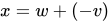
The equation is $v,w\in V$ uniquely solvable for all ; the solution is .

Examples

Euclidean plane

An illustrative vector space is the two-dimensional Euclidean plane $\mathbb R^2$ (in rectangular Cartesian coordinate systems) with the arrow classes (displacements or translations) as vectors and the real numbers as scalars.

$\vec v = ( 2 , 3 )$ is the shift of 2 units to the right and 3 units up,

$\vec w = ( 3 ,-5 )$ the shift by 3 units to the right and 5 units down.

The sum of two shifts is again a shift, and it is the shift obtained by performing the two shifts one after the other:

$\vec v + \vec w = ( 5 ,-2 )$ , i.e., shifting 5 units to the right and 2 units down.

The zero vector $\vec 0 = ( 0 , 0 )$ corresponds to the shift that leaves all points in place, i.e., the identical mapping.

Stretching the displacement ${\vec {v}}$ with a scalar a = 3 from the set of real numbers, we obtain three times the displacement:

$a \cdot \vec v = 3 \cdot ( 2 , 3 ) = ( 6 , 9 )$ .

Everything said about this example is also valid in the real affine plane.

Coordinate space

→ Main article: Coordinate space

If is a body and is a natural number, then the -fold Cartesian product forms

$K^{n}=\{(v_{1},\dots ,v_{n})\mid v_{1},\dots ,v_{n}\in K\},$

the set of all -tuples with entries in , a vector space over . Addition and scalar multiplication are defined component-wise; for $u=(u_{1},u_{2},\dots ,u_{n}),v=(v_{1},v_{2},\dots ,v_{n})\in K^{n}$ , α $\alpha \in K$ one sets:

$u + v = (u_1, u_2, \dots, u_n) + (v_1, v_2, \dots, v_n) = (u_1 + v_1, u_2 + v_2, \dots, u_n + v_n)$

and

$\alpha \cdot v=\alpha \cdot (v_{1},v_{2},\dots ,v_{n})=(\alpha \,v_{1},\alpha \,v_{2},\dots ,\alpha \,v_{n}).$

Often the -tuples are also notated as column vectors, that is, their entries are written one below the other. The vector spaces $K^{n}$ form, in a sense, the standard examples of finite-dimensional vector spaces. Every -dimensional -vector space is isomorphic to the vector space $K^{n}$ . Using a basis, each element of a vector space can be uniquely represented by an element of the $K^{n}$ coordinate tuple.

Function spaces

Principles and definition

→ Main article: Function space

If is a body, is a -vector space, and is an arbitrary set, then on the set F(A,V) of all functions $f \colon A \to V$ , addition and scalar multiplication can be defined pointwise: For 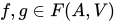$f, g \in F(A,V)$ and α $\alpha \in K$ , the functions $f + g \in F(A,V)$ and α are $\alpha \cdot f \in F(A,V)$ defined by.

(f + g) (x) = f(x) + g(x) for all $x\in A$ and

$(\alpha \cdot f) (x) = \alpha \cdot f(x)$ for all $x\in A$ .

With this addition and scalar multiplication, is F(A,V) a -vector space. In particular, this holds for F(A,K) , so if the target space is chosen to be the body itself. Further examples of vector spaces are obtained as subvector spaces of these function spaces.

In many applications, $K = \R$ , the body of real numbers, or $K=\mathbb {C}$ , the body of complex numbers, and is a subset of $\mathbb {R}$ , $\mathbb {R} ^{n}$ , $\mathbb {C}$ or $\mathbb {C} ^{n}$ . Examples include the vector space of all functions from $\mathbb {R}$ to $\mathbb {R}$ and the subspaces $C^0(\R,\R)$ of all continuous functions and $C^k(\R,\R)$ of all -times continuously differentiable functions from $\mathbb {R}$ to $\mathbb {R}$ .

Space of linear functions

A simple example of a function space is the two-dimensional space of real linear functions, that is, functions of the form

$f\colon\R\to\R,\;x\mapsto a x + b$

with real numbers and . These are those functions whose graph is a straight line. The set of these functions is a subvector space of the space of all real functions, because the sum of two linear functions is again linear, and a multiple of a linear function is also a linear function.

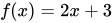
For example, the sum of the two linear functions and with

f(x) = 2x + 3 , g(x) = 3x - 5 ,

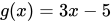the function f + g with

(f + g)(x) = f(x) + g(x) = 2x + 3 + 3x - 5 = (2+3)x + (3-5) = 5x - 2 .

The 3-fold of the linear function is the linear function with

$(3f)(x) = 3 \cdot f(x) = 3 \cdot (2x + 3) = (3 \cdot 2)x + (3 \cdot 3) = 6x + 9$ .

Polynomial Spaces

The set K[X] of polynomials with coefficients from a body forms, with the usual addition and the usual multiplication by a body element, an infinite-dimensional vector space. The set of monomials $\{1,\ x,\ x^2,\ x^3,\ x^4, \dots \}$ is a basis of this vector space. The set of polynomials whose degree is bounded by an $n\in \mathbb {N}$ is upper bounded, forms a subvector space of dimension n+1 . For example, the set of all polynomials of degree less than or equal to 4, that is, all polynomials of the form

ax^4 + b x^3 + c x^2 + d x + e ,

a 5-dimensional vector space with basis $\{1,\ x,\ x^2,\ x^3,\ x^4\}$ .

For infinite bodies one can identify the (abstract) polynomials with the associated polynomial functions. In this approach, the polynomial spaces correspond to subspaces of the space of all functions from to . For example, the space of all real polynomials of degree ≤ $\le 1$ corresponds to the space of linear functions.

Body enlargements

If is a superbody of then with its addition and the restricted multiplication $K\times L\rightarrow L$ as scalar multiplication is a -vector space. The rules to be proved for this follow directly from the body axioms for . This observation plays an important role in the theory of bodies.

For example, $\mathbb {C}$ in this way is a two-dimensional $\mathbb {R}$ -vector space; a basis is $\{1, \mathrm i\}$ . Similarly, $\mathbb {R}$ is an infinite-dimensional $\mathbb {Q}$ -vector space, but where a basis cannot be concretely specified.

{\displaystyle \sin +\exp :\mathbb {R} \to \mathbb {R} }

Author

AlegsaOnline.com Vector space Leandro Alegsa

URL: https://en.alegsaonline.com/art/104441

How to cite this article

APA

Alegsa, L. (April 23, 2026). Vector space. AlegsaOnline.com. https://en.alegsaonline.com/art/104441

MLA

Alegsa, Leandro. “Vector space.” AlegsaOnline.com, April 23, 2026, https://en.alegsaonline.com/art/104441

Chicago

Alegsa, Leandro. “Vector space.” AlegsaOnline.com. Updated April 23, 2026. https://en.alegsaonline.com/art/104441

BibTeX

@misc{alegsaonline_104441,
  author = {Alegsa, Leandro},
  title = {Vector space},
  year = {2026},
  howpublished = {AlegsaOnline.com},
  url = {https://en.alegsaonline.com/art/104441},
  note = {Updated: April 23, 2026; Language: en}
}

TXT

Leandro Alegsa. “Vector space.” AlegsaOnline.com. Updated: April 23, 2026. https://en.alegsaonline.com/art/104441