Variance

This article deals with the variance as a parameter of the distribution of a real random variable. For the variance of a sample, see sample variance; for other meanings, see variance.

The variance (Latin variantia "difference" or variare "(change), be different") is a measure of the dispersion of the probability density around its centre of gravity. Mathematically, it is defined as the mean square deviation of a real random variable from its expected value. It is the central second-order moment of a random variable.

The variance can be physically interpreted as a moment of inertia and can be determined with a variance estimator, e.g. the sample variance. The square root of the variance is the most important measure of dispersion in stochastics, known as the standard deviation.

The term "variance" was coined primarily by the British statistician Ronald Fisher (1890-1962). Other words for variance are the obsolete dispersion (Latin dispersio "dispersion" or dispergere "to distribute, spread out, scatter"), the scattering square or dispersion.

Properties of the variance include that it is never negative and does not change when the distribution is shifted. The variance of a sum of uncorrelated random variables is equal to the sum of their variances. A disadvantage of the variance for practical applications is that, unlike the standard deviation, it has a different unit from the random variable. Since it is defined by an integral, it does not exist for all distributions, i.e., it may be infinite.

A generalization of variance is covariance. Unlike variance, which measures the variability of the random variable under consideration, covariance is a measure of the joint variability of two random variables. From this definition of covariance, it follows that the covariance of a random variable with itself is equal to the variance of that random variable. In the case of a real random vector, the variance can be generalized to the variance-covariance matrix.

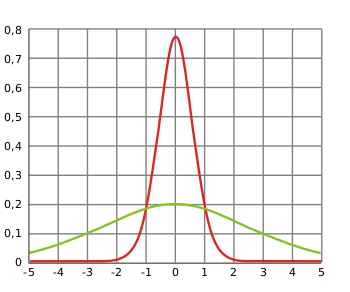
Density functions of two normally distributed random variables (red) and (green) with equal expected value μ $\mu _{X}=\mu _{Y}=0$ , but different variances. The horizontal axis shows the value, the vertical axis the frequency. Since the red curve f(x) narrower around the expected value than the green f(y) , it has a lower variance ( $\sigma _{X}^{2}<\sigma _{Y}^{2}$ ). The square root of the variance, the standard deviation, can be read from the turning points in the normal distribution.

Introduction to the problem

As a starting point for the construction of the variance, one considers an arbitrary quantity that is dependent on chance and can thus assume different values. This quantity, which is denoted by following, follows a certain distribution. The expected value of this variable is denoted by

$\mu :=\mathbb {E} (X)$

abbreviated. The expected value indicates the average value of the random variable . It can be interpreted as the center of gravity of the distribution (see also section Interpretation) and reflects its location. However, in order to sufficiently characterize a distribution, a quantity is missing which, as a key figure, provides information about the strength of dispersion of a distribution around its centroid. This quantity should always be greater than or equal to zero, since negative dispersion cannot be meaningfully interpreted. A first obvious approach would be to use the mean absolute deviation of the random variable from its expected value:

$\mathbb {E} \left(|X-\mu |\right)$ .

Since the magnitude function used in the definition of the mean absolute deviation is not differentiable everywhere, and otherwise sums of squares are usually used in statistics, it makes sense to use the mean squared deviation, i.e. the variance, instead of the mean absolute deviation.

Calculation of the variance

Variance for discrete random variables

A random variable with a finite or countably infinite range of values ${\mathcal {T}}=\{x_{1},x_{2},\dotsc ,x_{k},\dotsc \}$ is called discrete. Its variance is then calculated as the weighted sum of the squares of the deviations (from the expected value):

$\sigma ^{2}=(x_{1}-\mu )^{2}p_{1}+(x_{2}-\mu )^{2}p_{2}+\ldots +(x_{k}-\mu )^{2}p_{k}+\ldots =\sum _{i\geq 1}(x_{i}-\mu )^{2}p_{i}$ .

Here $p_{i}=P(X=x_{i})$ the probability that $x_{i}$ takes the value Thus, in the above sum, each possible expression $(x_{i}-\mu )^{2}$ is $p_{i}$ weighted by the probability of its occurrence Thus, for discrete random variables, the variance is a weighted sum with weights $p_{i}\;(i=1,\ldots ,n)$ . The expected value of a discrete random variable also represents a weighted sum given by

$\mu =x_{1}p_{1}+x_{2}p_{2}+\ldots +x_{k}p_{k}+\ldots =\sum _{i\geq 1}x_{i}p_{i}$

is given. The sums extend in each case over all values that this random variable can assume. In the case of a countably infinite range of values, the result is an infinite sum. In words, the variance, in the discrete case, is calculated as the sum of the products of the probabilities of the realizations of the random variable with the respective squared deviation.

Variance for continuous random variables

A random variable is said to be continuous if its value range is a countable quantity. If the random variable is absolutely continuous, then as a consequence of Radon-Nikodým's theorem there exists a probability density function (density for short) $f_{X}(x)$ . In the case of a real-valued random variable, the distribution function $F(t)=P(X\leq t)$ , $t\in \mathbb {R}$ , as an integral as follows:

$F(t)=\int _{-\infty }^{t}f(x)\,\mathrm {d} x$

For the variance of a real-valued random variable with density f(x) now holds

$\operatorname {Var} (X)=\int _{-\infty }^{\infty }(x-\mathbb {E} [X])^{2}f(x)\,\mathrm {d} x\quad$ , where its expected value is given by $\mathbb {E} [X]=\int _{-\infty }^{\infty }xf(x)\,\mathrm {d} x$ .

If a density exists, the variance is calculated as the integral over the product of the squared deviation and the density function of the distribution. Thus, it is integrated over the space of all possible expressions (possible value of a statistical characteristic).