
Transpose (matrix operation)
The transpose of a matrix or vector swaps rows and columns. This article explains the definition, basic properties, common notation, examples, and where the transpose is used in mathematics and applications.
Overview
The transpose is a basic linear-algebra operation that converts the rows of a matrix into columns and vice versa. For an m-by-n matrix A the transpose, written AT or A', is an n-by-m matrix whose (i,j) entry equals A's (j,i) entry. The same idea applies to vectors: a column vector becomes a row vector under transposition and vice versa. See also general material on matrices.
Image gallery
1 Image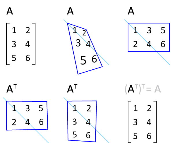
Definition and simple example
Formally, if A = (a_{ij}) then A^T = (a_{ji}). For instance, a 2×3 matrix can become a 3×2 matrix by swapping indices. If A = [[1,2,3],[4,5,6]] then A^T = [[1,4],[2,5],[3,6]]. Transposition is purely a reorganization of entries and does not change the underlying field of scalars.
Basic properties
- Involution: (A^T)^T = A.
- Linearity: (A+B)^T = A^T + B^T and (cA)^T = cA^T for scalars c.
- Product rule: (AB)^T = B^T A^T (note the reversal).
- Inverse: If A is invertible then (A^{-1})^T = (A^T)^{-1}.
Uses and examples
Transposition appears throughout linear algebra and applications: forming dot products (x^T y), describing symmetric matrices (A^T = A) and skew-symmetric matrices (A^T = -A), defining covariance matrices in statistics, and manipulating transformations in computer graphics. It is also used when changing between row-space and column-space viewpoints or when implementing algorithms that require particular memory layouts.
Variants and notable facts
For complex matrices the conjugate transpose (also called the Hermitian transpose and written A* or A^H) combines transposition with complex conjugation and is important for inner products and self-adjoint operators. Notation for the ordinary transpose varies: A^T, A', A^{tr} and others are all used in texts. Transpose is an easy operation conceptually but has important algebraic consequences because it reverses multiplication order and interacts with many structural matrix properties.


Terms and first properties
Notation
As notation, the arrangement of the elements in rows and columns between two large opening and closing brackets has become established. As a rule, round brackets are used, but square brackets are also used. For example
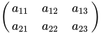 and
and 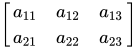
Matrices with two rows and three columns. Matrices are usually denoted by capital letters (sometimes bolded or, handwritten, single or double underlined), preferably  , denoted. A matrix with
  rows and
  columns:
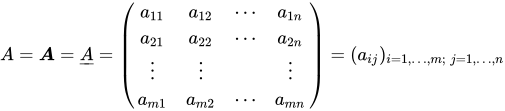 .
.
Elements of the matrix
The elements of the matrix are also called entries or components of the matrix. They originate from a set  usually a body or a ring. One speaks of a matrix over
  . If one chooses for the set of real numbers, one speaks of a real matrix, for complex numbers of a complex matrix.
A given element is described by two indices, usually the element in the first row and the first column is described by  . Generally,
  denotes the element in the
  -th row and the
  -th column. When indexing, the row index is always named first and the column index second. Rule of thumb: row first, column later. If there is a danger of confusion, the two indices are separated by a comma. For example, the matrix element in the first row and the eleventh column is named .
Individual rows and columns are often referred to as column or row vectors. Example:
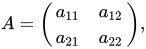 here
here  and
and  the columns or column vectors and
  and
and  the rows or row vectors.
For singly standing row and column vectors of a matrix, the invariant index is occasionally omitted. Sometimes column vectors are written as transposed row vectors for more compact representation, thus:
or  as
as 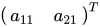 or
or 
Type
The type of a matrix is determined by the number of its rows and columns. A matrix with rows and columns is called an  matrix (speak: m-by-n or m-cross-n matrix). If the number of rows and columns match, it is called a square matrix.
A matrix consisting of only one column or only one row is usually considered a vector. A vector with elements can be represented as a single-column  matrix or a single-line
  matrix, depending on the context. In addition to the terms column vector and row vector, the terms column matrix and row matrix are common for this. A
  matrix is both a column and row matrix and is considered a scalar.
Formal representation
A matrix is a doubly indexed family. Formally this is a function

which assigns to each index pair  as function value the entry . For example, the index pair
  is assigned as a function value the entry
  . Thus, the function value is the entry in the -th row and the -th column. The variables and correspond to the number of rows and columns, respectively. Not to be confused with this formal definition of a matrix as a function is that matrices themselves describe linear mappings.
The set  of all -matrices over the set is also called in usual mathematical notation
  ; for this, the shorthand notation
  common. Sometimes the notations
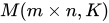 or more rarely
  used.
used.
Addition and multiplication
Elementary arithmetic operations are defined on the space of matrices.
Matrix addition
→ Main article: Matrix addition
Two matrices can be added if they are of the same type, that is, if they have the same number of rows and the same number of columns. The sum of two matrices is defined componentwise:

Calculation example:

In linear algebra, the entries of the matrices are usually elements of a body, such as the real or complex numbers. In this case, the matrix addition is associative, commutative, and has a neutral element in the form of the zero matrix. In general, however, the matrix addition has these properties only if the entries are elements of an algebraic structure that has these properties.
Scalar multiplication
→ Main article: Scalar multiplication
A matrix is multiplied by a scalar by multiplying each entry of the matrix by the scalar:

Calculation example:

Scalar multiplication must not be confused with scalar product. To be allowed to perform scalar multiplication, the scalar λ  (lambda) and the entries of the matrix must
  come from the same ring The set of -matrices in this case is a (left) module over
Matrix multiplication
→ Main article: Matrix multiplication
Two matrices can be multiplied if the number of columns of the left matrix is equal to the number of rows of the right matrix. The product of a  matrix
  and an matrix
  is an
is an  matrix
  whose entries are computed by applying the product sum formula, similar to the scalar product, to pairs of a row vector of the first matrix and a column vector of the second matrix:
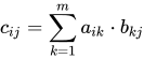
Matrix multiplication is not commutative, i.e., in general  . However, matrix multiplication is associative, i.e., it always holds:

Therefore, a chain of matrix multiplications can be parenthesized in different ways. The problem of finding a bracketing that leads to a computation with the minimum number of elementary arithmetic operations is an optimization problem. Moreover, matrix addition and matrix multiplication satisfy both distributive laws:

for all -matrices  and -matrices
  as well as

for all matrices and matrices 
Quadratic matrices  can be multiplied by themselves, analogous to the power in real numbers one introduces abbreviatively the matrix power
  or
or  . Thus it is also useful to insert square matrices as elements in polynomials. For further discussion on this, see Characteristic Polynomial. For simpler computation, the Jordan normal form can be used here. Quadratic matrices over
  or
or  can even be used in power series, cf. matrix exponential. A special role with respect to matrix multiplication is played by the square matrices over a ring
  , that is,
  . These themselves, with matrix addition and multiplication, in turn form a ring called a matrix ring.
Related articles
Author
AlegsaOnline.com Transpose (matrix operation) Leandro Alegsa
URL: https://en.alegsaonline.com/art/101200