
Transformation (mathematics)
A mathematical transformation is a rule that maps points between coordinate systems or within a space. It includes linear, affine, projective and non‑linear types and is central to geometry, physics, and computing.
Overview. In mathematics, a transformation is any rule or mapping that takes points or figures from one position or coordinate description to another. Transformations may act within a single space or relate different coordinate systems; for an explanation of coordinate frameworks see coordinate system. They can be expressed as formulas, functions, or operators and are studied both for their geometric effect and their algebraic representation.
Image gallery
5 Images
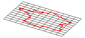

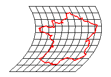

Representation and properties
Many transformations are written as functions f: X → Y that send each input point to an image point. In linear and affine settings these functions correspond to matrices (possibly with an added translation vector). Important properties include invertibility, fixed points, preservation of distance or angle, and behavior under composition. Repeated use of a transformation or composing several of them often yields another valid transformation, and collections of transformations with composition form algebraic structures such as groups and semigroups.
Common types
- Translations move every point by the same vector.
- Rotations turn points about an axis or center; see typical geometric rotation examples via rotation.
- Reflections flip a figure across a line or plane; basic mirror symmetries are described at reflection.
- Dilations (scalings) change sizes while preserving shape, and shears distort shapes by shifting layers parallel to a direction.
- Inversions and non‑linear mappings can swap interior and exterior regions, such as circle inversion in plane geometry.
History and development
The systematic algebraic study of transformations grew from the introduction of coordinate geometry, which allowed geometric motions to be encoded by equations. Later developments in linear algebra and group theory provided tools to classify and manipulate transformations; for example, the Erlangen program emphasized describing geometries by their transformation groups. Over time, transformations have been generalized from simple Euclidean motions to affine, projective, conformal, and more specialized maps used across mathematics.
Uses and significance
Transformations are fundamental across many fields. In geometry they describe symmetry and congruence; in physics they express changes of reference frame and conservation laws; in computer graphics they position and animate objects by matrices; in data analysis and machine learning they are used for feature scaling and dimensionality reduction. Robotics and engineering rely on transformations to model kinematics and sensor frames, while mapping and geographic information systems use coordinate transforms to reconcile different projections.
Distinctions and notable facts
Key distinctions include linear vs affine (affine adds translation), rigid vs similarity transformations (rigid preserves distances, similarity preserves shapes up to scale), and local vs global behavior for non‑linear maps. Determinants of associated matrices indicate orientation and volume scaling for linear maps. Understanding which properties a transformation preserves guides its application and classification in theory and practice.
For further context on coordinate representations, rotational conventions, or reflective symmetries see linked topics above or consult standard references on linear algebra and geometry.

Linear transformations
See also: Linear mapping
In linear transformations, the new coordinates are linear functions of the original ones, i.e.



 .
.
This can be compactly represented as a matrix multiplication of the old coordinate vector  with the matrix
 containing the coefficients
 .
.
The origin of the new coordinate system coincides with that of the original coordinate system.
Rotation
An important type of linear coordinate transformations are those in which the new coordinate system is rotated around the origin of the coordinates (the so-called "alias transformation" in the adjacent graphic). In two dimensions, the only parameter is the angle of rotation; in three dimensions, on the other hand, an axis of rotation that is not changed by the rotation must also be defined. The rotation is described in both cases by a rotation matrix.
Example
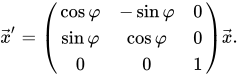
Consider two three-dimensional Cartesian coordinate systems  and
and  with a common z-axis and common origin. Let the coordinate system be rotated clockwise about the z-axis
 with respect to by an angleA point P that
  has coordinates the coordinate system S then has coordinates the coordinate system S'
 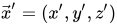 with:
with:



In matrix notation, the inverse rotation matrix for this rotation of the coordinate system gives:
Scaling
Scaling changes the "units" of the axes. That is, the numerical values of the coordinates  are
are  multiplied ("scaled") by constant factors λ

The parameters of this transformation are the  Numbers λ . A special case is the "scale transformation" where all factors have the same value

The matrix in this case is λ  times the unit matrix.
Shear
During shear, the angle between the coordinate axes changes. Therefore, in two dimensions there is one parameter, and in three-dimensional space - three parameters.


Affine transformations
See also: Affine mapping
Affine transformations consist of a linear transformation and a translation.
If both coordinate systems involved are linear, (i.e. in principle given by a coordinate origin and uniformly subdivided coordinate axes), then an affine transformation is present. Here the new coordinates are affine functions of the original ones, thus



This can be compactly written as matrix multiplication of the old coordinate vector with the matrix , containing the coefficients , and adding a vector {\displaystyle  containing the
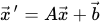
The translation is a special case of an affine transformation where A is the unit matrix.
Displacement (Translation)
Two coordinate systems and are considered. The system is shifted with respect to by the vector A point which 
 has coordinates in the coordinate system , then has coordinates the coordinate system
  .
.

Related articles
Author
AlegsaOnline.com Transformation (mathematics) Leandro Alegsa
URL: https://en.alegsaonline.com/art/101149